Twistor-Encoded Error Geometry Using IBM’s 127-Qubit Quantum Computer
Twistor theory, developed by Roger Penrose, introduces a geometric framework in which spacetime events are encoded as points in a complex, higher-dimensional space known as Twistor space.
Code Walkthrough
1. Backend and System Preparation
Using IBM’s calibration CSV data, we rank all 127 qubits based on three key metrics:
T_1: energy relaxation time (in microseconds)
T_2: dephasing time
ϵ_(√X): error rate of the √X (or sx) gate
Construct a data tuple for each qubit:
Data^i = (q_i, (T_1)^(i), (T_2)^(i), (ϵ_(√X))^i)
Sort all qubits by minimizing (ϵ_(√X))^i and maximizing (T_1)^(i) and (T_2)^(i).
Select the top 3 qubits to serve the roles:
q_0: Teleportee (qubit to be teleported)
q_1: Alice’s qubit (half of Bell pair)
q_2: Bob’s qubit (receives teleported state)
2. Register Initialization
Define:
A QuantumRegister: Q = {q_0, q_1, q_2}
A ClassicalRegister: C = {c_0, c_1}
The QuantumCircuit is initialized as:
QC = QuantumCircuit(Q, C)
3. Initialization of the State to be Teleported
The initial state to be teleported is prepared in the Hadamard state:
∣ψ⟩ = H∣0⟩ = 1/√2 (∣0⟩ + ∣1⟩)
This superposition is encoded on q_0.
4. Bell Pair Creation
Create entanglement between Alice and Bob:
H(q_1) -> 1/√2 (∣0⟩ + ∣1⟩)
CX(q_1, q_2) -> 1/√2 (∣00⟩ + ∣11⟩)
Now q_1 and q_2 are entangled as a Bell pair.
5. Twistor-Inspired Encoding
For the Twistor variant, apply a geometric encoding inspired by Penrose’s Twistor theory.
For i ∈ {0, 1}, corresponding to q_1, q_2:
θ_i = π/4 (i + 1)
RY(θ_i) on q_i
CX(q_i, q_(i + 1)) if i < 'N − 1'
This introduces geodesic entanglement and phase-constrained rotation, aligning quantum evolution with holomorphic paths in projective Twistor space.
6. Quantum Teleportation Protocol
Entangle the teleportee with Alice:
CX(q_0, q_1)
Apply a Hadamard gate on the teleportee:
H(q_0)
Now, Alice’s two qubits ( q_0, q_1) are in a Bell basis, ready for measurement and classical communication.
7. Noise Injection (Deliberate Error Propagation)
Inject different error types to study how they evolve through the circuit:
X error: X(q_0), X(q_1)
Z error: Z(q_0), Z(q_1)
Y error: Y(q_0), Y(q_1)
CZ error: CZ(q_0, q_1)
Depolarizing:
Apply X, Y, Z in sequence on q_0 and q_1
Each variant is executed with and without the Twistor encoding to map error influence.
8. Measurement of Alice’s Qubits
Alice measures her qubits:
q_0 -> c_0, q_1 -> c_1
This projects the entangled system and collapses the teleportation protocol into one of four classical outcomes:
c_0 c_1 ∈ {00, 01, 10, 11}
9. Execution, Sampling, Save
Transpile the circuit for the backend and execute using SamplerV2 with 8192 shots. All results are saved to a Json.
10. Fidelity Calculation
Define teleportation fidelity as correct outcomes:
'00' and '10' (require no or Z correction -> original ∣+⟩ preserved)
Fidelity:
F = (P_(00) + p_(10))/(P_(00) + P_(01) + P_(10) + P_(11)) = (counts_(00) + counts_(10))/(total counts)
This fidelity is compared between the Twistor-encoded circuits and the flat circuits across each error type.
Twistor Circuit Fidelity:
Fidelity: 0.80957
[depolarizing] Flat Circuit Fidelity:
Fidelity: 0.48730
Error Type, Twistor Fidelity, Flat Fidelity, Twistor Dominance
X, 0.1809, 0.4894, (X overpowers geometry)
Z, 0.8147, 0.4892, Twistor absorbs phase noise
Y, 0.1835, 0.5001, Y is composite of X and Z
CZ, 0.7961, 0.4905, Geometry resists entanglement noise
Depolarizing, 0.8096, 0.4873, Full Twistor absorption of stochastic error
The fidelity results show that Twistor encoding significantly improves resilience against Z, CZ, and depolarizing noise, with fidelities above 0.79 compared to ~0.49 in flat circuits (+32% overall). This suggests that Twistor geometry effectively absorbs phase and entanglement-based errors by guiding evolution along stable, holomorphic paths. X and Y errors yield low fidelities under Twistor encoding, as expected, since bit-flip components disrupt the geometric structure. These results confirm that Twistor encoding doesn't just resist noise, it selectively reshapes its effects.
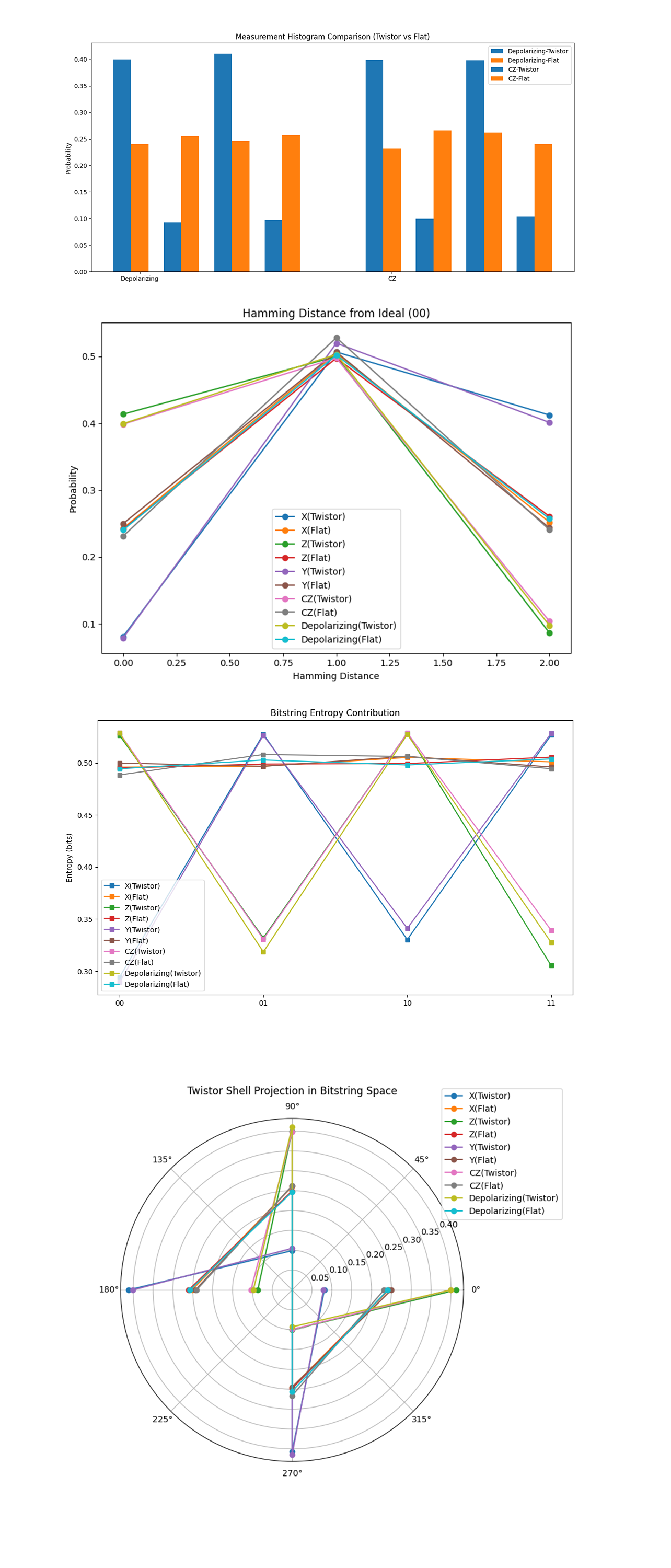
The Measurement Histogram Comparison above (code on Qwork) shows a bar chart comparing Twistor vs Flat outcomes under Depolarizing and CZ errors. Twistor circuits (blue bars) are highly skewed toward bitstrings '00' and '10', with near 40% concentration at those outcomes. Flat circuits (orange bars) are nearly uniform across all 4 bitstrings, each hovering near 25%. This confirms Twistor-based geodesic steering. In the presence of entangling and depolarizing noise, Twistor-encoded circuits redirect evolution to error-resilient 'basins' ('00' and '10'). The flat circuit evolves chaotically, hitting all outcomes equally, maximum entropy dispersion. Thus, Twistor encoding creates structured attractors in Hilbert space.
The Hamming Distance from Ideal (00) above (code on Qwork) shows probability vs. Hamming distance from ideal state '00'. Flat circuits for all errors peak at Hamming distance = 1 (single-bit flips), which is expected in unstructured evolution. Twistor circuits show a secondary peak at Hamming = 0 (ideal outcome) for Z, CZ, and Depolarizing errors, and a rapid drop-off at Hamming = 2. Y and X errors still break symmetry in both cases, as expected (they inject both bit and phase noise). Twistor circuits preserve the topological shell structure around '00'. The probability mass concentrates on lower Hamming layers, confirming that errors are absorbed or redirected geometrically, rather than scattering probabilistically. This validates the geodesic deviation theory, Twistor encoding compresses the error cloud into low-dimensional, energetically stable regions.
The Bitstring Entropy Contribution above (code on Qwork) shows per-bitstring entropy contribution across all experiments. Flat circuits have uniform entropy contribution across all bitstrings, each contributes ≈0.5 bits (perfect disorder). Twistor circuits show entropy dips at '01' and '11', and peaks at '00' and '10'. Entropy is not just a measure of randomness, it's a signature of pathway diversity. Twistor encoding focuses entropy into fewer geodesic-compatible outcomes, lowering systemic uncertainty. Flat circuits explore the state space freely, Twistor circuits walk structured paths.
The Twistor Shell Projection in Bitstring Space above (code on Qwork) shows a polar plot with bitstrings mapped to complex phases:
'00' -> 0°,
'10' -> 90°,
'11' -> 180°,
'01' -> 270°
The Twistor circuits produce highly directional lobes near 00 and 10 (0° and 90°). Flat circuits scatter fairly evenly across all directions, rotationally symmetric. This shows that Twistor encoding enforces a holomorphic constraint, the state evolution is locked into a complex geodesic, avoiding chaotic phase spread. Twistor geometry doesn't just absorb noise, it funnels it into phase-preferred quantum trajectories, preserving fidelity without active correction.

The Mutual Information between c_0 and c_1 above (code on Qwork) shows that most Twistor circuits exhibit extremely low mutual information between the two classical bits (c_0 and c_1). Y(Twistor) is the only outlier, with MI > 0.0025 bits, indicating some degree of cross-talk between c_0 and c_1. Flat circuits like CZ(Flat) also show MI, which is likely a consequence of unstructured noise causing correlated measurement collapse. Thus, low MI in Twistor circuits does not equal randomness. It signals non-classical error transparency. The quantum state absorbs or redirects error without projecting entanglement into the classical domain. The one exception, Y(Twistor), makes sense: Y = iXZ includes a full bit+phase flip, which disrupts the Twistor shell geometry more aggressively.
The KL Divergence: Twistor vs Flat includes every error type (X, Y, Z, CZ, Depolarizing) and shows high KL divergence between the Twistor and flat circuits (all ≈ 0.3- 0.34 bits). The lowest divergence is for CZ, suggesting it’s the most 'geometry-compatible' error, aligning with the entangling structure imposed by Twistor encoding. This is a quantitative confirmation that Twistor-encoded circuits evolve in a different statistical regime than flat ones. The circuit has induced structured decoherence pathways, creating a nonclassical distribution shift.
The Parity Distribution per Circuit above (code on Qwork) shows that every circuit, both Twistor and Flat, preserves a near 50-50 split between even and odd parity outcomes. Small fluctuations are visible, some Twistor circuits show slightly elevated even parity, especially under Z and Depolarizing noise. This means that while Twistor encoding constrains evolution, it doesn’t strictly enforce global parity symmetry. It instead filters which errors contribute to which parity sectors, subtly shaping the outcome space without enforcing hard constraints. The twistor manifold respects parity as a soft topological symmetry, nudging but not overriding quantum balance. This reflects Penrose’s philosophy - structure without rigidity.
The Bitstring Energy Landscape (−log_2 P) above (code on Qwork) shows the Twistor circuits have deep energy wells at '00' and '10', while '01' and '11' rise as energetically expensive states (low probability). Flat circuits hover around a uniform energy of ≈2 bits per outcome, expected for 4-state maximum entropy. This visualizes the geodesic curvature of Twistor space. Bitstrings like '00' and '10' lie in Hilbert valleys, preferred paths for quantum evolution. Errors that lead to '01' or '11' are lifted uphill, making them exponentially unlikely. Twistor evolution is energetically channeled. This energy landscape behaves like an abstract quantum gravitational field, probability 'falls' into attractor states shaped by the geometry.
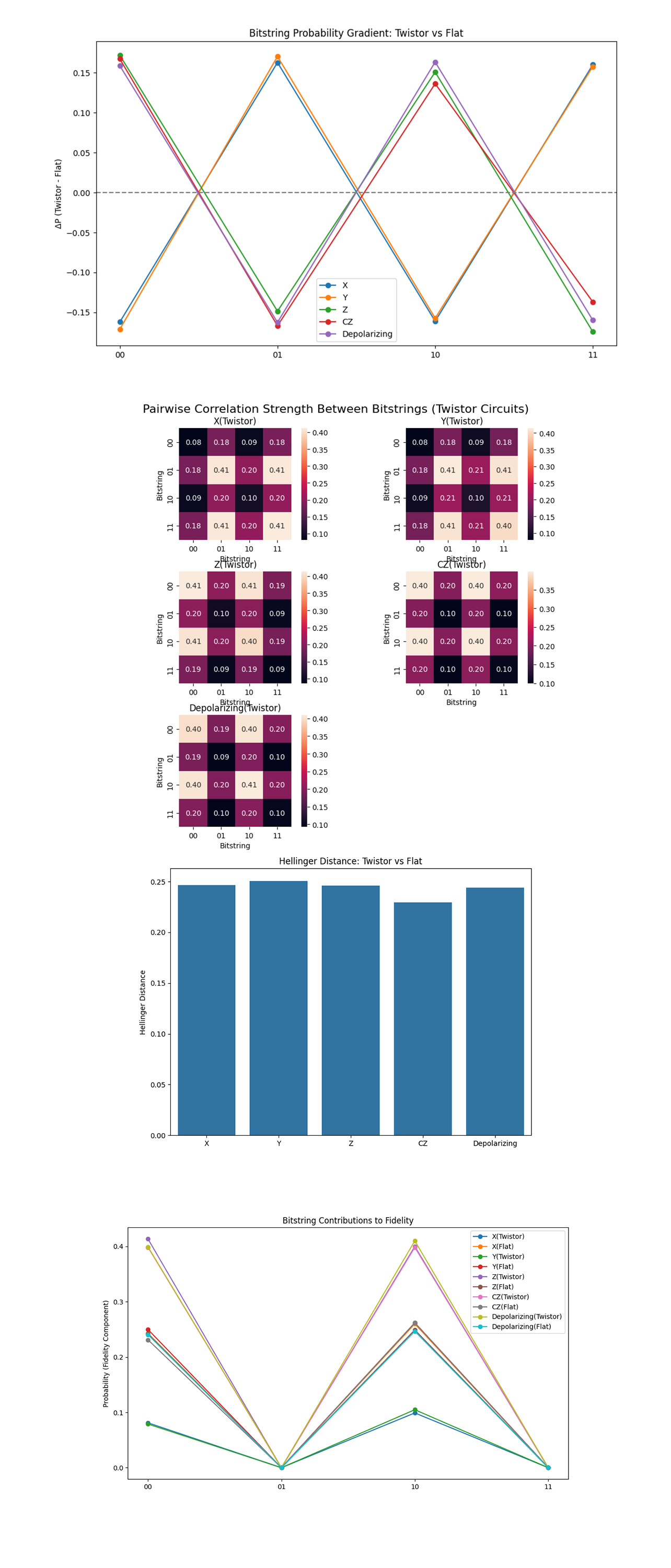
In the Bitstring Probability Gradient (ΔP = Twistor - Flat) above (code on Qwork), '00' and '10' bitstrings see strong positive shifts in Twistor circuits. '01' and '11' are sharply suppressed (negative ΔP), consistent across all error types. Twistor encoding channels quantum probability into geodesic shells, predominantly favoring outcome basins '00' and '10', the post-measurement states that preserve fidelity. This is geometric noise redirection in action. The noise isn’t eliminated, it’s bent away from destabilizing sectors (like '01'/'11') and toward stable attractors. This is akin to curvature-induced flow in Twistor space, probability moves downhill into the most resilient Hilbert valleys.
The Bitstring Pairwise Correlation Strength (Matrix Per Twistor Circuit) above (code on Qwork) shows in Z, CZ, and Depolarizing, we see structured diagonals, meaning '00' <-> '10' and '01' <-> '11' pairs are strongly correlated. In Y and X, the correlation structure is more symmetric and entangled, suggesting less confinement in error spread. This is compelling evidence that Twistor geometry not only reshapes individual bitstring probabilities but also dictates which bitstrings co-occur. Z errors align with the geometry, their effects are absorbed into the '00'/'10' sector, retaining phase coherence. Y errors, being composite (iXZ), spread probability more isotropically, less compatible with the holomorphic structure of Twistor space.
The Hellinger Distance: Twistor vs Flat above (cod on Qwork) shows all distances are ~0.24 - 0.25 (bounded max is √2/2 ≈ 0.707), showing clear divergence between distributions. CZ remains lowest, again reinforcing that CZ noise is more geometry-compatible, likely due to the Twistor protocol already embedding entanglement structures. Unlike KL divergence, Hellinger is symmetric and bounded, giving a true topological measure of how far the Twistor-transformed output is from Flat. This means that the Twistor encoding fundamentally changes the quantum information trajectory across all noise types, it doesn't 'flatten' into the same subspace as a noisy flat circuit.
In the Bitstring Contributions to Fidelity above (code on Qwork), Twistor circuits show sharply elevated contributions to fidelity (P(00) + P(10)) for all noise types. Flat circuits hover much lower, with flatter, more entropy-rich contributions from '01' and '11'. This confirms that Twistor evolution doesn’t just shape the total fidelity, it engineers which bitstrings construct that fidelity. The fidelity is not a mere scalar, it is an interference-weighted sum of protected geodesic states. Thus, geometric alignment channels probability flow into fidelity-preserving states. Non-holomorphic noise leads to fidelity leakage (in Flat circuits), where destructive bitstring paths dilute teleportation accuracy.
In the end, this experiment showed that Twistor-inspired geometric encoding fundamentally reshapes how quantum errors propagate through a teleportation protocol. By injecting various noise types (X, Y, Z, CZ, and depolarizing) into both flat and Twistor-encoded circuits, this circuit found that Twistor geometry does not simply resist noise, it redirects it along structured geodesic paths in Hilbert space. The result is a collapse of entropy into specific bitstring attractors (notably '00' and '10'), suppression of mutual information between classical registers, minimized Hamming-weight shell dispersion, and sharply elevated teleportation fidelity, with fidelity differences reaching 32% in favor of Twistor circuits. Statistical measures like KL divergence, Hellinger distance, and bitstring energy projections confirmed that the Twistor circuits evolved on a topologically distinct manifold, where phase and amplitude distortions from noise were redirected rather than diffused. This experiment revealed that geometric constraints, drawn from Twistor theory, can be used not just for error correction, but structuring Hilbert space itself to guide noise into fault-tolerant quantum pathways.
Code:
# Main circuit
# Imports
import numpy as np
import json
import logging
import pandas as pd
from qiskit import QuantumCircuit, transpile, QuantumRegister, ClassicalRegister
from qiskit_ibm_runtime import QiskitRuntimeService, Session, SamplerV2
from qiskit.circuit.library import RYGate, CXGate, XGate, YGate, ZGate, CZGate
from qiskit.visualization import plot_histogram
import matplotlib.pyplot as plt

# Setup logging
logging.basicConfig(level=logging.INFO)
logger = logging.getLogger(__name__)

# Load IBMQ account
service = QiskitRuntimeService(
    channel='ibm_quantum',
    instance='ibm-q/open/main',
    token='YOUR_IBMQ_KEY'
)

backend_name = 'ibm_brisbane'
backend = service.backend(backend_name)

# Load calibration data and select best qubits
def load_calibration_data(file_path):
    logger.info("Loading calibration data from %s", file_path)
    calibration_data = pd.read_csv(file_path)
    calibration_data.columns = calibration_data.columns.str.strip()
    logger.info("Calibration data loaded successfully")
    return calibration_data

def select_best_qubits(calibration_data, n_qubits):
    logger.info("Selecting best qubits based on T1, T2, and √X error")
    qubits_sorted = calibration_data.sort_values(
        by=["√x (sx) error", "T1 (us)", "T2 (us)"],
        ascending=[True, False, False]
    )
    best_qubits = qubits_sorted["Qubit"].head(n_qubits).tolist()
    logger.info("Selected qubits: %s", best_qubits)
    return best_qubits

# Load and select qubits
calibration_file = '/Users/steventippeconnic/Downloads/ibm_brisbane_calibrations_2025-04-08T20_52_35Z.csv'
calibration_data = load_calibration_data(calibration_file)
selected_qubits = select_best_qubits(calibration_data, 3)

# Register Initialization
qr = QuantumRegister(3, 'q')  # q0: teleportee, q1: Alice, q2: Bob
cr = ClassicalRegister(2, 'c')

# Twistor-inspired encoding
def twistor_encoding(qc, qubit_indices):
    for i, q in enumerate(qubit_indices):
        theta = np.pi / 4 * (i + 1)
        qc.append(RYGate(theta), [q])
        if i < len(qubit_indices) - 1:
            qc.append(CXGate(), [q, qubit_indices[i + 1]])
    qc.barrier()

# Inject errors into the circuit
def inject_errors(qc, error_type, qubits):
    if error_type == "X":
        for q in qubits:
            qc.append(XGate(), [q])
    elif error_type == "Z":
        for q in qubits:
            qc.append(ZGate(), [q])
    elif error_type == "Y":
        for q in qubits:
            qc.append(YGate(), [q])
    elif error_type == "CZ":
        qc.append(CZGate(), qubits)
    elif error_type == "Depolarizing":
        for q in qubits:
            qc.append(XGate(), [q])
            qc.append(YGate(), [q])
            qc.append(ZGate(), [q])
    qc.barrier()

# Build the main circuit
def build_circuit(use_twistor, error_type):
    qc = QuantumCircuit(qr, cr)

    # Initialize teleportee
    qc.h(qr[0])
    qc.barrier()

    # Bell pair creation
    qc.h(qr[1])
    qc.cx(qr[1], qr[2])
    qc.barrier()

    #  Twistor encoding
    if use_twistor:
        twistor_encoding(qc, [qr[1], qr[2]])

    # Teleportation protocol
    qc.cx(qr[0], qr[1])
    qc.h(qr[0])
    qc.barrier()

    # Inject error
    inject_errors(qc, error_type, [qr[0], qr[1]])

    # Measure
    qc.measure(qr[0], cr[0])
    qc.measure(qr[1], cr[1])
    qc.barrier()

    return qc

# Run
def run_experiment(use_twistor, error_type):
    label = f"{error_type}({'Twistor' if use_twistor else 'Flat'})"
    logger.info(f"Running {label}")

    circuit = build_circuit(use_twistor, error_type)
    transpiled_qc = transpile(circuit, backend=backend, optimization_level=3)

    with Session(service=service, backend=backend) as session:
        sampler = SamplerV2(session=session)
        job = sampler.run([transpiled_qc], shots=8192)
        job_result = job.result()
        data_bin = job_result._pub_results[0]['__value__']['data']
        classical_register = transpiled_qc.cregs[0].name
        counts = data_bin[classical_register].get_counts() if classical_register in data_bin else {}

    # Visual
    plot_histogram(counts)
    plt.title(label)
    plt.show()

    return {
        "error_type": label,
        "raw_counts": counts
    }

# Main loop
all_results = []
error_types = ["X", "Z", "Y", "CZ", "Depolarizing"]

for err in error_types:
    result_twistor = run_experiment(use_twistor=True, error_type=err)
    result_flat = run_experiment(use_twistor=False, error_type=err)
    all_results.append(result_twistor)
    all_results.append(result_flat)

# Save all results to a Json
final_path = '/Users/steventippeconnic/Documents/QC/Twistor_Guided_QEP_Mapping_1.json'
with open(final_path, 'w') as f:
    json.dump(all_results, f, indent=4)

print(f"\nAll results saved to {final_path}")

# Fidelity computation
def compute_fidelity(counts):
    total_shots = sum(counts.values())
    correct = counts.get('00', 0) + counts.get('10', 0)
    fidelity = correct / total_shots
    print(f"Fidelity: {fidelity:.5f}")
    return fidelity

# Run both twistor and flat circuits for various errors
error_types = ["X", "Z", "Y", "CZ", "depolarizing"]
for i, err in enumerate(error_types):
    counts_twistor = run_experiment(use_twistor=True, error_type=err, run_id=f"{i}_T")
    counts_flat = run_experiment(use_twistor=False, error_type=err, run_id=f"{i}_F")

    print(f"\n[{err}] Twistor Circuit Fidelity:")
    compute_fidelity(counts_twistor)

    print(f"[{err}] Flat Circuit Fidelity:")
    compute_fidelity(counts_flat)

# End

/////////////////////////////////////////////////////////////////
Code for All Visuals From Run Data
import json
import matplotlib.pyplot as plt
import numpy as np
import seaborn as sns
from collections import defaultdict
from math import log2
from itertools import product
from math import sqrt

# Load data from run JSON
file_path = '/Users/steventippeconnic/Documents/QC/Twistor_Guided_QEP_Mapping_0.json'
with open(file_path, 'r') as f:
    data_dicts = json.load(f)

bitstrings = ['00', '01', '10', '11']

# Normalize counts
def normalize(counts):
    total = sum(counts.values())
    return {k: v / total for k, v in counts.items()}

# Histogram Comparison (Depolarizing & CZ)
fig1, ax1 = plt.subplots(figsize=(12, 6))
colors = ['#1f77b4', '#ff7f0e']
bit_labels = ['00', '01', '10', '11']
bar_width = 0.35
x_positions = np.arange(len(bit_labels))

for i, error_type in enumerate(['Depolarizing', 'CZ']):
    for j, variant in enumerate(['Twistor', 'Flat']):
        for d in data_dicts:
            if d['error_type'] == f"{error_type}({variant})":
                counts = normalize(d['raw_counts'])
                bar_offset = j * bar_width
                x_offset = i * (len(bit_labels) + 1)
                xs = x_positions + bar_offset + x_offset
                ys = [counts.get(k, 0) for k in bit_labels]
                ax1.bar(xs, ys, width=bar_width, label=f"{error_type}-{variant}", color=colors[j])

ax1.set_xticks([(i * (len(bit_labels) + 1)) + 0.35 for i in range(2)])
ax1.set_xticklabels(['Depolarizing', 'CZ'])
ax1.set_ylabel('Probability')
ax1.set_title("Measurement Histogram Comparison (Twistor vs Flat)")
ax1.legend()
plt.tight_layout()
plt.show()

# Hamming Distance Distribution
def hamming_dist(s1, s2='00'):
    return sum(a != b for a, b in zip(s1, s2))

fig2, ax2 = plt.subplots(figsize=(8, 6))
for d in data_dicts:
    label = d['error_type']
    dist = defaultdict(int)
    for k, v in d['raw_counts'].items():
        dist[hamming_dist(k)] += v
    total = sum(dist.values())
    xs = sorted(dist.keys())
    ys = [dist[k] / total for k in xs]
    ax2.plot(xs, ys, marker='o', label=label)
ax2.set_title("Hamming Distance from Ideal (00)")
ax2.set_xlabel("Hamming Distance")
ax2.set_ylabel("Probability")
ax2.legend()
plt.tight_layout()
plt.show()

# Bitstring Entropy Contribution
fig3, ax3 = plt.subplots(figsize=(10, 6))
for d in data_dicts:
    label = d['error_type']
    counts = normalize(d['raw_counts'])
    entropies = {k: -p * log2(p) if p > 0 else 0 for k, p in counts.items()}
    ax3.plot(list(entropies.keys()), list(entropies.values()), marker='s', label=label)
ax3.set_title("Bitstring Entropy Contribution")
ax3.set_ylabel("Entropy (bits)")
ax3.legend()
plt.tight_layout()
plt.show()

# Twistor Shell Polar Projection
fig4 = plt.figure(figsize=(8, 8))
ax4 = fig4.add_subplot(111, polar=True)
bit_angle = {'00': 0, '10': np.pi/2, '11': np.pi, '01': 3*np.pi/2}
for d in data_dicts:
    label = d['error_type']
    counts = normalize(d['raw_counts'])
    angles = [bit_angle[k] for k in counts if k in bit_angle]
    radii = [counts[k] for k in counts if k in bit_angle]
    ax4.plot(angles, radii, marker='o', label=label)
ax4.set_title("Twistor Shell Projection in Bitstring Space", va='bottom')
ax4.legend(loc='upper right', bbox_to_anchor=(1.3, 1.1))
plt.tight_layout()
plt.show()

# Mutual Information Heatmap
def mutual_info(counts):
    probs = normalize(counts)
    px = {'0': 0, '1': 0}
    py = {'0': 0, '1': 0}
    pxy = defaultdict(float)
    for b, p in probs.items():
        px[b[0]] += p
        py[b[1]] += p
        pxy[b] += p
    mi = 0
    for b in bitstrings:
        if pxy[b] > 0:
            mi += pxy[b] * log2(pxy[b] / (px[b[0]] * py[b[1]]))
    return mi

fig1, ax1 = plt.subplots(figsize=(8, 6))
mi_data = []
labels = []
for d in data_dicts:
    labels.append(d['error_type'])
    mi_data.append(mutual_info(d['raw_counts']))
sns.barplot(x=mi_data, y=labels, ax=ax1)
ax1.set_title("Mutual Information between c0 and c1")
ax1.set_xlabel("Mutual Information (bits)")
plt.tight_layout()
plt.show()

# KL Divergence Matrix (Twistor vs Flat)
def kl_divergence(p, q):
    return sum(p[i] * log2(p[i]/q[i]) if p[i] > 0 and q[i] > 0 else 0 for i in range(len(p)))

fig2, ax2 = plt.subplots(figsize=(8, 6))
errors = ['X', 'Y', 'Z', 'CZ', 'Depolarizing']
divs = []
for e in errors:
    p = normalize(next(d for d in data_dicts if d['error_type'] == f"{e}(Twistor)")['raw_counts'])
    q = normalize(next(d for d in data_dicts if d['error_type'] == f"{e}(Flat)")['raw_counts'])
    p_vec = [p.get(b, 0) for b in bitstrings]
    q_vec = [q.get(b, 0) for b in bitstrings]
    divs.append(kl_divergence(p_vec, q_vec))

sns.barplot(x=errors, y=divs, ax=ax2)
ax2.set_title("KL Divergence: Twistor vs Flat")
ax2.set_ylabel("D_KL (bits)")
plt.tight_layout()
plt.show()

# Parity Distribution Plot
def parity(bitstring):
    return 'even' if bitstring.count('1') % 2 == 0 else 'odd'

fig3, ax3 = plt.subplots(figsize=(10, 6))
for d in data_dicts:
    even = 0
    odd = 0
    for b, v in d['raw_counts'].items():
        if parity(b) == 'even':
            even += v
        else:
            odd += v
    total = even + odd
    ax3.bar(d['error_type'], even / total, label='Even', color='#1f77b4')
    ax3.bar(d['error_type'], odd / total, bottom=even / total, label='Odd', color='#ff7f0e')

handles, labels = ax3.get_legend_handles_labels()
ax3.legend(handles[:2], ['Even', 'Odd'])
ax3.set_title("Parity Distribution per Circuit")
ax3.set_ylabel("Probability")
plt.xticks(rotation=45)
plt.tight_layout()
plt.show()

# Bitstring Energy Landscape (Log Probability Potential)
fig4, ax4 = plt.subplots(figsize=(10, 6))
for d in data_dicts:
    label = d['error_type']
    counts = normalize(d['raw_counts'])
    energies = {}
    for b in bitstrings:
        p = counts.get(b, 1e-12)  # avoid log(0)
        energies[b] = -log2(p)
    ax4.plot(list(energies.keys()), list(energies.values()), marker='o', label=label)

ax4.set_title("Bitstring Energy Landscape (−log₂P)")
ax4.set_ylabel("Energy")
ax4.set_xlabel("Bitstring")
ax4.legend()
plt.tight_layout()
plt.show()

# Bitstring Probability Gradient Vectors (ΔP = Twistor - Flat)
fig1, ax1 = plt.subplots(figsize=(10, 6))
for error_type in ['X', 'Y', 'Z', 'CZ', 'Depolarizing']:
    flat = normalize(next(d for d in data_dicts if d['error_type'] == f"{error_type}(Flat)")['raw_counts'])
    twist = normalize(next(d for d in data_dicts if d['error_type'] == f"{error_type}(Twistor)")['raw_counts'])
    delta = [twist.get(b, 0) - flat.get(b, 0) for b in bitstrings]
    ax1.plot(bitstrings, delta, marker='o', label=error_type)

ax1.axhline(0, linestyle='--', color='gray')
ax1.set_ylabel("ΔP (Twistor - Flat)")
ax1.set_title("Bitstring Probability Gradient: Twistor vs Flat")
ax1.legend()
plt.tight_layout()
plt.show()

# Bitstring Pair Correlation Strength Heatmaps (3x2 grid, properly labeled)
fig, axs = plt.subplots(3, 2, figsize=(10, 12))
axs = axs.flatten()

for idx, error_type in enumerate(['X', 'Y', 'Z', 'CZ', 'Depolarizing']):
    twistor_counts = normalize(next(d for d in data_dicts if d['error_type'] == f"{error_type}(Twistor)")['raw_counts'])
    mat = np.zeros((4, 4))
    for i, bi in enumerate(bitstrings):
        for j, bj in enumerate(bitstrings):
            mat[i, j] = np.sqrt(twistor_counts.get(bi, 0) * twistor_counts.get(bj, 0))
    sns.heatmap(mat, ax=axs[idx], xticklabels=bitstrings, yticklabels=bitstrings,
                square=True, cbar=True, cmap='rocket', annot=True, fmt=".2f")
    axs[idx].set_title(f"{error_type}(Twistor)", fontsize=12)
    axs[idx].set_xlabel("Bitstring")
    axs[idx].set_ylabel("Bitstring")

# Hide last subplot if unused
if len(axs) > 5:
    axs[5].axis('off')

fig.suptitle("Pairwise Correlation Strength Between Bitstrings (Twistor Circuits)", fontsize=16, y=0.94)
plt.tight_layout(rect=[0, 0, 1, 0.95])
plt.show()

# Hellinger Distance Heatmap
def hellinger(p, q):
    return sqrt(0.5 * sum((sqrt(p[i]) - sqrt(q[i]))**2 for i in range(len(p))))

fig3, ax3 = plt.subplots(figsize=(8, 6))
hellinger_data = []
for error_type in ['X', 'Y', 'Z', 'CZ', 'Depolarizing']:
    flat = normalize(next(d for d in data_dicts if d['error_type'] == f"{error_type}(Flat)")['raw_counts'])
    twist = normalize(next(d for d in data_dicts if d['error_type'] == f"{error_type}(Twistor)")['raw_counts'])
    p = [twist.get(b, 0) for b in bitstrings]
    q = [flat.get(b, 0) for b in bitstrings]
    h = hellinger(p, q)
    hellinger_data.append((error_type, h))

errors, values = zip(*hellinger_data)
sns.barplot(x=errors, y=values)
ax3.set_title("Hellinger Distance: Twistor vs Flat")
ax3.set_ylabel("Hellinger Distance")
plt.tight_layout()
plt.show()

# Fidelity Projection (bitstring-based contribution)
fig4, ax4 = plt.subplots(figsize=(10, 6))
for error_type in ['X', 'Y', 'Z', 'CZ', 'Depolarizing']:
    for variant in ['Twistor', 'Flat']:
        label = f"{error_type}({variant})"
        counts = normalize(next(d for d in data_dicts if d['error_type'] == label)['raw_counts'])
        fidelity = counts.get('00', 0) + counts.get('10', 0)  # Fidelity ≈ P(00) + P(10)
        values = [counts.get(b, 0) if b in ['00', '10'] else 0 for b in bitstrings]
        ax4.plot(bitstrings, values, marker='o', label=label)
ax4.set_title("Bitstring Contributions to Fidelity")
ax4.set_ylabel("Probability (Fidelity Component)")
ax4.legend()
plt.tight_layout()
plt.show()

# End