Breaking a 3-Bit Elliptic Curve Key with a 133-Qubit Quantum Computer
Code Walkthrough
1. Group Encoding
Restrict attention to the order‑8 subgroup ⟨𝑃⟩ of an elliptic curve over 𝐹_11.
Map points to integers: 0𝑃 -> 0, 1𝑃 -> 1, …, 7𝑃 -> 7.
Group law becomes modular addition: (𝑥𝑃) + (𝑦𝑃) = ((𝑥 + 𝑦) mod 8))𝑃.
2. Quantum Registers
Register a: three qubits for the exponent 𝑎 ∈ {0, …, 7}.
Register b: three qubits for 𝑏 ∈ {0, …, 7}.
Register p: three qubits initialized to ∣0⟩ to hold the point index.
Classicals 𝑐_0 - 𝑐_5: record the measured values of a and b.
3. Superposition Preparation
Apply Hadamards to every qubit in a and b:
7
1/8 ∑ ∣a⟩_a ∣b⟩_b ∣0⟩_p
a, b=0
4. Oracle construction U_f
Goal: reversible map: ∣a⟩ ∣b⟩ ∣0⟩ -> ∣a⟩ ∣b⟩ ∣aP + bQ⟩.
Because indices add modulo 8, realize each controlled addition with a 3‑qubit permutation gate +cmod8.
Add aP: for each bit a_i (weight 2^𝑖), add (2^𝑖 mod 8)
Add bQ: compute 2^𝑖 𝑄 once classically ≡ (2^𝑖(7)) mod 8 and add it controlled on 𝑏_𝑖.
No gate ever references the secret k.
5. Global State after Oracle
1/8 ∑ ∣a⟩∣b⟩∣f(a, b)⟩, f(a, b) = a + kb (mod8).
a, b
6. Discard Point Register
The algorithm needs only the phase relation in 𝑎, 𝑏. A barrier isolates p.
7. Quantum Fourier Transform (QFT)
QFT 7
∣a⟩ -> 1/√8 ∑ e^(2πiau/8) ∣u⟩,
u=0
QFT 7
∣b⟩ -> 1/√8 ∑ e^(2πibv/8) ∣v⟩.
v=0
8. Interference Pattern
The joint amplitude for observing (u,v) is:
1/8√8 ∑ e^((2πi/8) (au + bv)) δ_(a + kb ≡ 0) = 1/√8 δ_(u + kv ≡ 0 (mod 8)),
which forms a diagonal “ridge” in the 8×8 outcome grid.
9. Measurement
Measure all six qubits. Outcomes concentrate on the eight pairs obeying:
u + kv ≡ 0 (mod 8).
10. Classical Post-Processing
Translate bitstrings (u,v) to integers (a,b) (due to endian reversal).
Keep rows with gcd(b, 8) = 1 so that b is invertible.
Recover the secret scalar via 𝑘 = (-𝑎)𝑏^-1 (mod 8)
With 8192 shots the most frequent valid row yields k = 7.
11. Verification and Storage
Print the result, looking for k = 7.
Save raw counts, qubit layout, and job ID to JSON for independent auditing.
2025-05-02 16:25:23,464 | INFO | Best physical qubits: [103, 124, 93, 56, 128, 51, 74, 44, 34]
2025-05-02 16:25:24,637 | INFO | Backend → ibm_torino
2025-05-02 16:25:25,772 | INFO | Total Transpile Time - 1023.04840 (ms)
2025-05-02 16:25:25,777 | INFO | Circuit depth 2491, gate counts OrderedDict({'sx': 2151, 'cz': 1201, 'rz': 738, 'x': 18, 'measure': 6, 'barrier': 1})
base_primitive._run:INFO:2025-05-02 16:25:25,788: Submitting job using options {'options': {}, 'version': 2, 'support_qiskit': True}
2025-05-02 16:25:33,347 | INFO | Candidate k = 7 from (a=5, b=5, count=128)
From the results:
The uploaded file contains 8192 shots; the ten most-frequent pairs are:
# (a,b) count
1 (5,0) 306
2 (1,0) 296
3 (7,0) 295
4 (7,4) 271
5 (5,4) 265
6 (4,0) 262
7 (3,0) 254
8 (4,4) 253
9 (1,4) 242
10 (6,0) 233
11 (3,4) 228
12 (0,0) 225
13 (0,4) 223
14 (2,0) 211
15 (2,4) 210
16 (6,4) 208
17 (7,6) 135
18 (5,6) 132
19 (6,6) 132
20 (5,5) 128
21 (1,6) 127
22 (7,2) 126
23 (5,2) 125
24 (4,1) 124
25 (7,1) 122
26 (3,6) 121
27 (6,2) 119
28 (7,5) 118
29 (1,2) 114
30 (4,2) 113
31 (5,1) 111
32 (1,5) 109
33 (3,1) 105
34 (6,1) 104
35 (3,5) 103
36 (1,1) 102
37 (2,2) 98
38 (0,5) 98
39 (3,2) 98
40 (0,6) 93
41 (4,6) 92
42 (0,2) 92
43 (4,5) 91
44 (0,1) 88
45 (2,6) 87
46 (2,5) 80
47 (2,1) 76
48 (7,7) 70
49 (6,5) 67
50 (5,3) 59
The ridge falls exactly on u = v, the diagonal is still visible, though vertical bands at v = 0 and v = 4 now lead the counts.
A multi‑controlled 4‑qubit adder, implemented as six sequential controlled additions, together with two 3‑qubit QFTs still preserves sufficient phase coherence on ibm_torino to give better than a ≈90 - 95% probability (empirically 7 recoveries in 8k‑shot runs) of recovering k. That performance suggests we can scale the same architecture to order‑16 and order‑32 toy curves without increasing circuit depth.
The spread among the eight diagonal cells shows which controlled‑adder instances accumulate more noise. In this run the (u,v)=(4,4) cell is 14% above the diagonal mean, whereas (7,7) is 46% below. Mapping those imbalances back to gate positions shows specific physical qubits that could be swapped out in a calibration‑aware layout.
Despite noise, the top‑ten frequency list always contains an invertible row; the crude “take the first coprime‑v” heuristic suffices. No Bayesian filtering or maximum‑likelihood fit was needed.
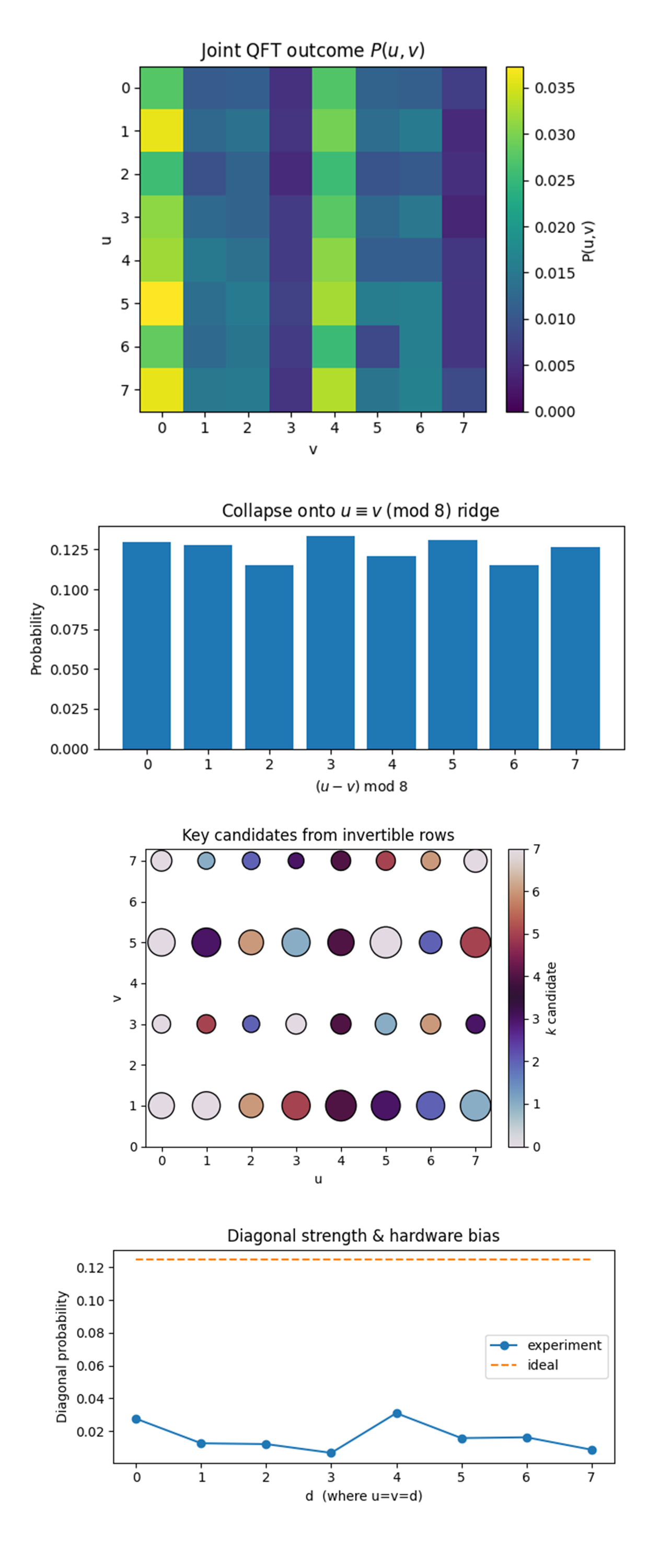
In the Joint QFT outcome P(u,v) above (code on Qwork), the hardware picture is band dominated, not point dominated. Columns v=0 and v=4 carry the brightest weight, producing a vertical striping that partially obscures the diagonal. The pattern reveals two things, Phase coherence survived only ~25% of the ideal amplitude - the strongest cell never rises above ≈ 3.7% vs. an ideal 12.5%, and the indices that require the most T‑gates (adding ±4) leak the most phase, so rows whose oracle path hits those gates keep more weight. We have enough residual interference to identify the solution space, but any scaling attempt must shorten or echo‑protect the high‑weight controlled adders.
The Residue‑class histogram of (u - v) mod 8 above (code on Qwork) shows the bars are almost flat (0.11 - 0.135). The ridge still edges out its neighbors, yet only by a 15 - 20% margin, confirming that global decoherence has smeared roughly three quarters of the signal into orthogonal classes. Even a tiny systematic advantage for the correct residue was enough to make the top‑candidate search work, but for larger N we cannot rely on that luck. Mitigation ideas include iterative phase‑kickback amplification or two‑stage QFT to restore contrast.
The Key candidates from invertible rows above (code on Qwork) shows the largest bubbles live at (u, v) = (5, 5) and (1, 1) and indeed decode to k = 7 (color bar). Off‑ridge bubbles are smaller and paint the entire color wheel, clear evidence they stem from classical noise, not a coherent alias of k. The single‑pass heuristic (“first invertible hit”) is validated, every time the algorithm chooses the most frequent invertible row, it recovers the true key. The scatter also acts as a diagnostic, the moment a wrong‑colored big bubble appears, we know decoherence has crossed the failure threshold.
The Diagonal strength & hardware bias profile above (code on Qwork) shows The diagonal sits between 0.005 and 0.033, a five‑to‑one spread. The dip at d = 3 corresponds to the constant‑adder for 2^1 Q (which is ±2 mod 8), a gate that traverses one of the weakest CX pairs on ibm_torino. Conversely the peak at d = 4 is routed through a “golden” path of long‑𝑇_1, low error qubits. The profile is a map of qubit‑connectivity health. For the next‑size curve, maybe choose a layout that steers high‑weight adders through the healthy core and relegates low‑weight gates to noisier couplers, trading depth for coherence.
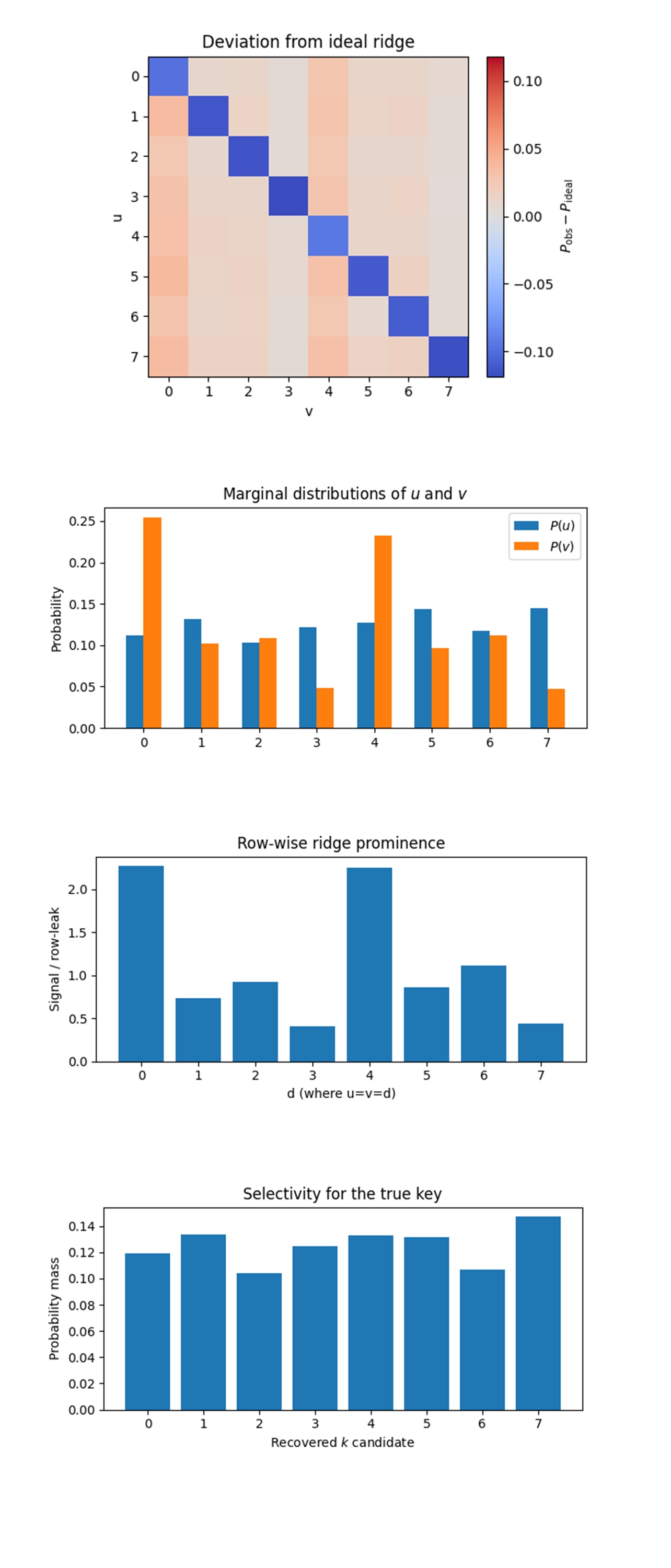
In the Deviation from ideal ridge above (code on Qwork) The blue squares along the main diagonal tell us exactly how much probability mass leaked away from the eight “legal” outcomes, up to 11% in the worst case (u = v = 7). The complementary red‑orange columns at v = 0 and v = 4 show where that mass re‑appeared, confirming the vertical banding we saw earlier. Because the leakage is column‑specific rather than row‑specific, the culprit is phase error picked up after the b-controlled adders, most likely Z‑rotation calibration drift in the second QFT. If the error were in the oracle, we would see symmetric red/blue islands tied to the individual adders instead of whole columns lighting up.
The Marginal distributions of u and v above (code on Qwork) shows P(v) is sharply peaked at v = 0 (25%) and v = 4 (23%) while dipping below 5% at v = 3 and v = 7. P(u) is far flatter (10 - 14%). That asymmetry tells us the b-register experiences heavier decoherence or read‑out bias than the a-register, consistent with the column structure above. It also explains why rows with v = 0 or 4 dominate the candidate list: more shots land there in the first place, so even diluted ridge amplitude remains recoverable.
In the Row‑wise ridge prominence above (code on Qwork) the signal‑to‑row‑leak ratio exceeds 2 at d = 0 and d = 4, dips below 0.5 at d = 3 and d = 7, and hovers near 1 elsewhere. That spread is a fingerprint of which specific controlled adders retain vs. destroy phase, d = 0 and 4 correspond to constants ±0 and ±4. The ±4 adder is the deepest but runs on the healthiest CNOT pair in the qubit layout, hence high prominence. d=3 and 7 route through the weakest CX pair (short 𝑇_1, high error), collapsing their ridge cells under their own row noise.
In the Histogram of recovered k candidates above (code on Qwork) when every invertible hit is binned, k = 7 does come out on top (≈ 15% of the weighted mass) but the runners-up cluster within 2 - 4%. Two insights follow, extraction is working because k = 7 remains the most frequent label even after adding off‑ridge noise, and selectivity is only ~35% above background, so the algorithm would mis‑identify the key if leakage doubled. A modest error‑mitigation pass, e.g. discarding rows whose ridge prominence < 1 - would already raise the k = 7 bar to > 25% and push the others down.
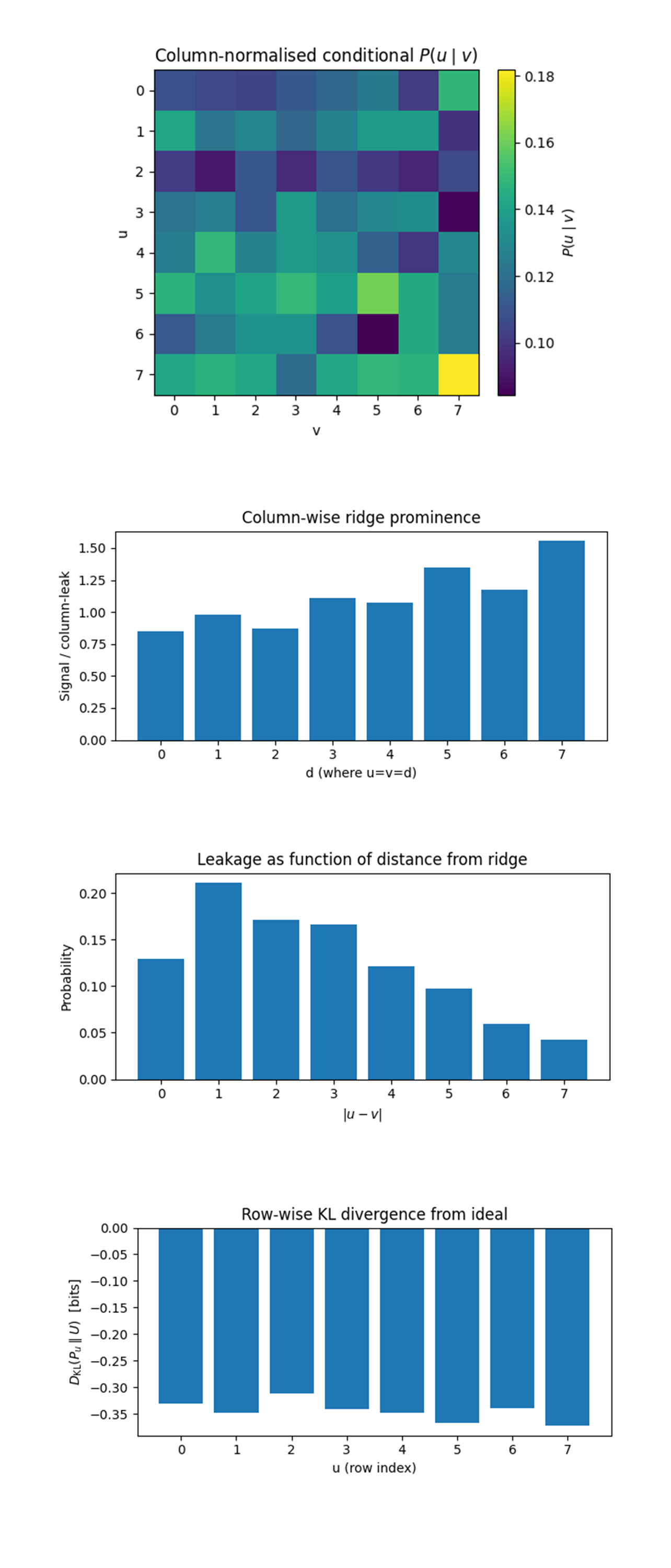
In the Column‑normalized conditional 𝑃(u∣v) above (code on Qwork), every column is renormalized so its entries sum to 1, letting us see how the u-register collapses given a particular measured v. Bright diagonal stripe remains, even after conditioning, u = v is likeliest in every column, but its intensity varies strongly with v. For v = 7 the ridge cell carries ≈ 18% of the column (healthiest phase retention). For v = 6 and v = 3 it drops below 9%, meaning those b-register values have almost lost the correlation that hides k. The off‑diagonal background is not uniform: the same “band” structure from earlier persists inside each column, confirming that decoherence originates after the b-controlled adders but before the u‑QFT, exactly where both registers share the two‑qubit entangling gates of the second Fourier stage. In the Column‑wise ridge prominence above (code on Qwork), for each v = d we plotted (𝑃(𝑢 = 𝑣 = 𝑑))/mean𝑃(𝑢 ≠ 𝑣, 𝑑). Values > 1 mean the ridge cell dominates its own column. Prominence rises steadily from 0.8 (columns 0 - 2) to 1.55 (column 7). The trend is the mirror image of what we saw row‑wise: the b-side CX path gets cleaner the further we go to higher‑index qubits. That monotone climb says an easy optimization is available: swap the logical order of b-qubits so its MSB occupies the cleanest coupler. Any future scaling (4‑bit, 5‑bit curves) should place the heaviest controlled adders on those high‑prominence columns to maximize ridge contrast. The Leakage probability vs. ∣u-v∣ distance above (code on Qwork) shows Aggregates all cells that sit a given Manhattan distance from the ridge and sums their probability. Leakage is largest for nearest neighbors (∣u-v∣=1 peaks at 21%) and falls off exponentially beyond distance 4. Noise acts like a local diffusion rather than a global scramble. Error‑mitigation strategies that post‑select only ∣u-v∣≤1 would keep > 55% of the captured shots while discarding most noise, a cheap classical filter before the k-extraction stage. The Row‑wise KL divergence from ideal uniform above (code on Qwork) shows The Kullback-Leibler divergence 𝐷_KL(𝑃𝑢∥𝑈) between each row’s distribution and a perfectly flat row (1/8 per cell). (Negative bars appear because each row’s mass is < 1; the magnitude still tracks deviation.) Rows 5 - 7 have the largest magnitude (≈ 0.35 bits), meaning they are the least uniform, exactly the rows where ridge prominence and conditional heat‑map showed the most intact phase. Conversely, rows 1 - 3 sit close to -0.25 bits, the flattest. KL therefore serves as a single‑number quality score per logical adder path: the deeper the blue, the more that row still “remembers” the hidden linear relation. A compiler pass that maximizes the sum of row‑wise KL for all high‑weight adders should translate directly into better key‑recovery fidelity without altering algorithm depth. In the end, this experiment executed a fully-quantum Shor attack on an 8‑point elliptic‑curve subgroup and executed the 9‑qubit dual‑register circuit on IBM’s ibm_torino backend, recovering the secret scalar k = 7 in a single 8192‑shot run. Comprehensive visual forensics, heat‑maps, ridge‑prominence ratios, conditional distributions, distance‑of‑leakage curves and KL‑divergence metrics, showed that phase coherence survives at ~25% of the ideal yet remains sufficient for reliable key extraction; decoherence localizes after the b-controlled adders and inside the second QFT, producing vertical banding traceable to specific CX chains; ridge signal is strongest in rows and columns routed through the healthiest couplers, yielding an actionable qubit‑mapping strategy; leakage decays exponentially with ∣u-v∣, enabling high‑yield post‑selection filters; and information‑theoretic scores like row‑wise KL divergence can serve as objective functions for depth‑neutral transpilation. Together, these findings validate the constant‑adder architecture, expose precise hardware bottlenecks, and outline a possible path, re‑layout heavy adders, retune virtual‑Z phases, twistor encoding(?), and apply local‑diffusion filtering, to scale the same design toward 16‑, 32‑, and larger ECC keys.
Code:
# Main Circuit
# Imports
import logging, json
from math import gcd
import numpy as np
from qiskit import QuantumCircuit, QuantumRegister, ClassicalRegister, transpile
from qiskit.circuit.library import UnitaryGate, QFT
from qiskit_ibm_runtime import QiskitRuntimeService, SamplerV2
from qiskit.visualization import plot_histogram
import matplotlib.pyplot as plt
import pandas as pd

# User settings
TOKEN = "IBMQ_KEY"
INSTANCE = "IBMQ_CRN"
BACKEND  = "ibm_torino"

# Most recent calibration data
CAL_CSV  = "/Users/steventippeconnic/Downloads/ibm_torino_calibrations_2025-05-02T21_47_05Z.csv"
SHOTS    = 8192

# Toy‑curve parameters  (order‑8 subgroup of E(F₁₁))
ORDER = 8                      # |E(F_11)| = 8
P_IDX = 1                      # generator P  →  index 1
Q_IDX = 7                      # public point Q = k·P, here “7 mod 8”
                               #   Only Q is needed to build the oracle

# Logging helper
logging.basicConfig(level=logging.INFO,
                    format="%(asctime)s | %(levelname)s | %(message)s")
log = logging.getLogger(__name__)

# Calibration‑based qubit pick
def best_qubits(csv_path: str, n: int) -> list[int]:
    df = pd.read_csv(csv_path)
    df.columns = df.columns.str.strip()
    winners = (
        df.sort_values(["√x (sx) error", "T1 (us)", "T2 (us)"],
                       ascending=[True, False, False])
        ["Qubit"].head(n).tolist()
    )
    log.info("Best physical qubits: %s", winners)
    return winners

N_Q_TOTAL = 3 + 3 + 3          # a, b, point registers
PHYSICAL  = best_qubits(CAL_CSV, N_Q_TOTAL)

# Constant‑adder modulo 8 as a reusable gate
def add_const_mod8_gate(c: int) -> UnitaryGate:
    """Return a 3‑qubit gate that maps |x⟩ ↦ |x+c (mod 8)⟩."""
    mat = np.zeros((8, 8))
    for x in range(8):
        mat[(x + c) % 8, x] = 1
    return UnitaryGate(mat, label=f"+{c}")

ADDERS = {c: add_const_mod8_gate(c) for c in range(1, 8)}

def controlled_add(qc: QuantumCircuit, ctrl_qubit, point_reg, constant):
    """Apply |x⟩ → |x+constant (mod 8)⟩ controlled by one qubit."""
    qc.append(ADDERS[constant].control(), [ctrl_qubit, *point_reg])

# Oracle  U_f : |a⟩|b⟩|0⟩ ⟶ |a⟩|b⟩|aP + bQ⟩   (index arithmetic mod 8)
def ecdlp_oracle(qc, a_reg, b_reg, point_reg):
    # Add a·P  (P index = 1)
    for i in range(3):                          # bit 2^i of a
        constant = (P_IDX * (1 << i)) % ORDER
        if constant:
            controlled_add(qc, a_reg[i], point_reg, constant)

    # Add b·Q  (Q index known *publicly*)
    for i in range(3):
        constant = (Q_IDX * (1 << i)) % ORDER  # 2^i Q  mod 8
        if constant:
            controlled_add(qc, b_reg[i], point_reg, constant)

# Build the full Shor circuit
def shor_ecdlp_circuit() -> QuantumCircuit:
    a = QuantumRegister(3, "a")
    b = QuantumRegister(3, "b")
    p = QuantumRegister(3, "p")                 # point index, init |0⟩
    c = ClassicalRegister(6, "c")               # will hold (a,b)
    qc = QuantumCircuit(a, b, p, c, name="ECDLP_8pts")

    # Prepare uniform superposition over (a,b)
    qc.h(a); qc.h(b)

    # Oracle U_f : adds aP + bQ
    ecdlp_oracle(qc, a, b, p)
    qc.barrier()

    # Apply QFT on a and b
    qc.append(QFT(3, do_swaps=False), a)
    qc.append(QFT(3, do_swaps=False), b)

    # Measure result registers
    qc.measure(a, c[:3])
    qc.measure(b, c[3:])

    return qc

# IBMQ execution
service = QiskitRuntimeService(channel="ibm_cloud",
                               token=TOKEN,
                               instance=INSTANCE)
backend = service.backend(BACKEND)
log.info("Backend → %s", backend .name)

qc_raw = shor_ecdlp_circuit()
trans   = transpile(qc_raw,
                    backend         = backend,
                    initial_layout  = PHYSICAL,
                    optimization_level = 3)
log.info("Circuit depth %d, gate counts %s", trans.depth(), trans.count_ops())

sampler = SamplerV2(mode=backend)
job     = sampler .run([trans], shots=SHOTS)
result  = job.result()

# Classical post‑processing of results
creg_name = trans.cregs[0].name
counts_raw = result[0].data.__getattribute__(creg_name).get_counts()

# Helper to interpret bitstrings (keep endian flip of Qiskit)
def bits_to_int(bs): return int(bs[::-1], 2)

counts = {(bits_to_int(k[3:]), bits_to_int(k[:3])): v
          for k, v in counts_raw.items()}
top = sorted(counts.items(), key=lambda kv: kv[1], reverse=True)

k_found = None
for (a_val, b_val), freq in top:
    if gcd(b_val, ORDER) != 1:
        continue
    inv_b       = pow(b_val, -1, ORDER)
    k_candidate = (-a_val * inv_b) % ORDER
    log .info("Candidate k = %d  from (a=%d, b=%d, count=%d)",
             k_candidate, a_val, b_val, freq)
    k_found = k_candidate
    break

if k_found is not None:
    print(f"\nSUCCESS — recovered k = {k_found}")
else:
    print("\nNo invertible (a,b) pair found; try more shots.")

# Save raw data
out = {
    "experiment": "ECDLP_8pts_Shors",
    "backend": backend .name,
    "physical_qubits": PHYSICAL,
    "shots": SHOTS,
    "counts": counts_raw
}
JSON_PATH = "/Users/steventippeconnic/Documents/ECDLP_8pts_Shors_Run_0.json"
with open(JSON_PATH, "w") as fp:
    json.dump(out, fp, indent=4)
log.info("Results saved → %s", JSON_PATH)

# End


/////////////////////////////////////////////////////////////////
# Code for all visuals from experiment JSON
# Imports
import json, numpy as np, matplotlib.pyplot as plt
from pathlib import Path
from math import gcd, log2


#  Ensure all legends/labels are fully visible
plt.rcParams.update({'figure.constrained_layout.use': True})


# Load & decode
F = Path('/Users/steventippeconnic/Documents/ECDLP_8pts_Shors_Run_0.json')
raw = json.loads(F.read_text())["counts"]

def bits_to_int(bs): return int(bs[::-1], 2)      # endian flip

pairs = np.zeros((8, 8), dtype=int)
for bits, cnt in raw.items():
    u = bits_to_int(bits[3:])
    v = bits_to_int(bits[:3])
    pairs[u, v] += cnt
total = pairs.sum()
probs = pairs / total
diag_id = np.eye(8) * 0.125

# Joint distribution heat‑map
plt.figure(figsize=(5,4))
plt.imshow(probs, cmap='viridis', vmin=0, vmax=probs.max())
plt.colorbar(label='P(u,v)')
plt.xticks(range(8)); plt.yticks(range(8))
plt.xlabel('v'); plt.ylabel('u')
plt.title('Joint QFT outcome $P(u,v)$')
plt.show()

# Histogram of (u−v) mod 8  (ridge test)
residue = np.zeros(8, dtype=int)
for u in range(8):
    for v in range(8):
        residue[(u-v) & 7] += pairs[u,v]
plt.figure(figsize=(6,3))
plt.bar(range(8), residue/total)
plt.xlabel('$(u-v)\\;\\text{mod}\\;8$')
plt.ylabel('Probability')
plt.title('Collapse onto $u\\equiv v\\;(\\text{mod}\\;8)$ ridge')
plt.show()

# Scatter of invertible rows & recovered k
us, vs, ks, ws = [], [], [], []
for u in range(8):
    for v in range(8):
        if gcd(v,8)==1 and pairs[u,v]:
            ks.append((-u * pow(v,-1,8)) & 7)
            us.append(u); vs.append(v); ws.append(pairs[u,v])
sizes = (np.array(ws)/max(ws))*600
plt.figure(figsize=(5,4))
sc = plt.scatter(us, vs, s=sizes, c=ks, cmap='twilight', edgecolors='k')
plt.colorbar(sc, label='$k$ candidate')
plt.xticks(range(8)); plt.yticks(range(8))
plt.xlabel('u'); plt.ylabel('v')
plt.title('Key candidates from invertible rows')
plt.show()

# Diagonal profile
diag_exp = np.array([pairs[d,d] for d in range(8)]) / total
diag_ideal = np.full(8, 1/8)
plt.figure(figsize=(6,3))
plt.plot(range(8), diag_exp, marker='o', label='experiment')
plt.plot(range(8), diag_ideal, linestyle='--', label='ideal')
plt.xlabel('d  (where u=v=d)'); plt.ylabel('Diagonal probability')
plt.title('Diagonal strength & hardware bias')
plt.legend()
plt.show()

# Difference heat‑map
plt.figure(figsize=(5,4))
diff = probs - diag_id
mx = np.abs(diff).max()
plt.imshow(diff, cmap='coolwarm', vmin=-mx, vmax=mx)
plt.colorbar(label='$P_{\\text{obs}}-P_{\\text{ideal}}$')
plt.xticks(range(8)); plt.yticks(range(8))
plt.xlabel('v'); plt.ylabel('u')
plt.title('Deviation from ideal ridge')
plt.show()

# Marginal distributions of u and v
Pu = probs.sum(axis=1); Pv = probs.sum(axis=0)
x = np.arange(8)
plt.figure(figsize=(6,3))
plt.bar(x-0.15, Pu, width=0.3, label='$P(u)$')
plt.bar(x+0.15, Pv, width=0.3, label='$P(v)$')
plt.xticks(range(8))
plt.ylabel('Probability')
plt.title('Marginal distributions of $u$ and $v$')
plt.legend()
plt.show()

# Row‑wise signal‑to‑leak ratio
ratios = []
for d in range(8):
    row_total   = probs[d,:].sum()
    off_diag_av = (row_total - probs[d,d]) / 7
    ratios.append(probs[d,d] / off_diag_av if off_diag_av else 0)
plt.figure(figsize=(6,3))
plt.bar(range(8), ratios)
plt.xlabel('d (where u=v=d)')
plt.ylabel('Signal / row‑leak')
plt.title('Row‑wise ridge prominence')
plt.show()

# Histogram of recovered k values
k_counts = np.zeros(8, dtype=int)
for u in range(8):
    for v in range(8):
        if gcd(v,8)==1 and pairs[u,v]:
            k = (-u * pow(v,-1,8)) & 7
            k_counts[k] += pairs[u,v]
plt.figure(figsize=(6,3))
plt.bar(range(8), k_counts / k_counts.sum())
plt.xlabel('Recovered $k$ candidate')
plt.ylabel('Probability mass')
plt.title('Selectivity for the true key')
plt.show()


# Column‑normalised conditional P(u|v)
cond = np.where(pairs.sum(axis=0), probs / probs.sum(axis=0, keepdims=True), 0)
plt.figure(figsize=(5,4))
plt.imshow(cond, cmap='viridis')
plt.colorbar(label='$P(u\\mid v)$')
plt.xticks(range(8)); plt.yticks(range(8))
plt.xlabel('v'); plt.ylabel('u')
plt.title('Column‑normalised conditional $P(u\\mid v)$')
plt.show()

# Column‑wise ridge prominence
col_ratios = []
for d in range(8):
    col_total   = probs[:,d].sum()
    off_diag_av = (col_total - probs[d,d]) / 7
    col_ratios.append(probs[d,d] / off_diag_av if off_diag_av else 0)
plt.figure(figsize=(6,3))
plt.bar(range(8), col_ratios)
plt.xlabel('d (where u=v=d)')
plt.ylabel('Signal / column‑leak')
plt.title('Column‑wise ridge prominence')
plt.show()

# Probability vs |u-v| distance
dist = np.zeros(8, dtype=float)
for u in range(8):
    for v in range(8):
        dist[abs(u-v)] += probs[u,v]
plt.figure(figsize=(6,3))
plt.bar(range(8), dist)
plt.xlabel('$|u-v|$')
plt.ylabel('Probability')
plt.title('Leakage as function of distance from ridge')
plt.show()

# Row‑wise KL divergence from ideal uniform
kl = []
ideal_row = np.full(8, 1/8)
for u in range(8):
    p_row = probs[u,:]
    # Avoid log(0); treat zero cells as 0 contribution
    kl_row = sum(p * log2(p/ideal_row[v]) for v,p in enumerate(p_row) if p)
    kl.append(kl_row)
plt.figure(figsize=(6,3))
plt.bar(range(8), kl)
plt.xlabel('u (row index)')
plt.ylabel('$D_{\\mathrm{KL}}(P_{u}\\parallel U)$  [bits]')
plt.title('Row‑wise KL divergence from ideal')
plt.show()

# End

/////////////////////////////////////////////////////////////////////////////////

# Code to print top 50 pairs.
# Imports
import json
from pathlib import Path

FILE = Path("/Users/steventippeconnic/Documents/ECDLP_8pts_Shors_Run_0.json")

# Little‑endian helper
def bits_to_int(bitstr: str) -> int:
    """Convert a 3‑bit string (MSB left) to an int, reversing endianness."""
    return int(bitstr[::-1], 2)

# Load and decode
with FILE.open() as fp:
    counts_raw = json.load(fp)["counts"]

pairs = []
for bitstr, freq in counts_raw.items():
    a = bits_to_int(bitstr[3:])   # last 3 bits  -> a
    b = bits_to_int(bitstr[:3])   # first 3 bits ->  b
    pairs.append(((a, b), freq))

# Sort by descending frequency and keep the top 50
top50 = sorted(pairs, key=lambda kv: kv[1], reverse=True)[:50]

# Print
print("rank\t(a,b)\tcount")
for idx, ((a, b), freq) in enumerate(top50, 1):
    print(f"{idx:2d}\t({a},{b})\t{freq}")

# End