Nonlocal Ridge Encryption via Modular Interference on Two 5-Qubit Registers Using IBM’s 156-Qubit Quantum Computer ibm_fez

This experiment demonstrates a toy-scale interference-based encryption primitive in which the ciphertext is not stored in any single quantum register but emerges from nonlocal correlations between registers. Executed on IBM's 156-qubit ibm_fez using qiskit Runtime 2.0, the circuit encodes a masked secret scalar k into a joint quantum state over two 5-qubit registers using a modular group-phase relation a ≡ k′ b (mod 32). Neither marginal distribution reveals the encoded value; instead, k′ becomes recoverable only from the joint measurement statistics, where quantum interference produces a structured ridge in the 32 x 32 outcome space. A classical mask separates the recoverable ciphertext k′ from the true secret k. From 8192 shots, the experiment produces a stable, hardware-resilient deviation of P(a,b) from P(A)P(B), demonstrating that information can be encoded in global interference geometry rather than in local observables. This provides a minimal, hardware-realized example of nonlocal interference-based encryption.
All Backend Data ZIP Download
Paper Version Download

Code Walkthrough

1. Choose parameters and define the modular space
Choose a small toy modulus of the form
N = 2^n, n = 5 -> N = 32.
All arithmetic on the registers a and b is interpreted modulo 32.
Choose:
the true secret k (what we ultimately want to hide),
a mask r (classical offset),
and the cipher-slope:
k′ ≡ k + r (mod 32).
In the concrete run:
k = 13, r = 6, k′ = 13 + 6 = 19 (mod 32).
Note: This is a toy-scale primitive intended to study information geometry, not a secure encryption scheme.

2. Enforce invertibility for decoding from correlations
Later, to recover a slope from measured pairs, we need to divide by b (multiply by its modular inverse). In modulus 2^n, only odd numbers are invertible, so restrict attention to outcomes where:
gcd(b,2^n) = 1 (b is odd)
Separately, choose k′ to be odd so that multiplication by k′ is bijective over Z_(2^n). This ensures that the map:
B ↦ a = k' b (mod 2^n)
is a permutation, helping keep the marginals high-entropy and approximately uniform.
In the concrete run, k′ = 19 is odd, satisfying this design choice.

3. Define the quantum registers and the intended nonlocal relation
Allocate two n-qubit registers:
b: 5 qubits (the input share),
a: 5 qubits (the output share),
so the total quantum system is 10 qubits.
The target functional relation we want embedded into the joint quantum state is:
a ≡ k′ b (mod 32).
This relation is the ridge, outcomes lie on a modular line in the discrete (a,b) grid.

4. Prepare b in a uniform superposition
Initialize the system in ∣0⟩^(⊗10).
Apply Hadamards to all qubits of register b, producing:
∣b⟩ -> 1/√32 (∑_b=0)^31 ∣b⟩.
So the joint state becomes:
∣a = 0⟩ ⊗ 1/√32 (∑_b=0)^31 ∣b⟩.

5. Compute the modular multiplication a <- k′ b (mod 32)
Now implement a reversible arithmetic computation that maps:
∣a⟩ ∣b⟩ -> ∣a + k′ b (mod 32)⟩ ∣b⟩.
Since a starts at 0, this produces:
∣0⟩ ⊗ 1/√32 (∑_b=0)^31 ∣b⟩ -> 1/√32 (∑_b=0)^31 ∣k′ b mod 32⟩ ∣b⟩.
This is the key nonlocal encoding, no single register contains the secret slope by itself, it is expressed in the correlation between them.
The arithmetic identity used:
Write b in binary:
b = (∑_j=0)^(n−1) b_j 2^j, 𝑏_𝑗 ∈ {0, 1}
Then:
k′ b ≡ (∑_j=0)^(n−1) b_j (k′ 2^j) (mod 2^n).
So modular multiplication can be built from a sequence of controlled modular adds of constants k′ 2^j.

6. Implement modular adds using the Quantum Fourier Transform (QFT)
To make modular addition efficient in gate form, add in Fourier space.
Apply QFT on register a:
The Quantum Fourier Transform over 2^n is:
QFT ∣x⟩ = 1/√2^n (∑_y=0)^(2^n-1) e^(2πixy/2^n) ∣y⟩.
Apply QFT to a so that additions to a can be performed by phase rotations.
Add constants with controlled phase rotations:
Adding a constant c to a register in Fourier space corresponds to applying phase shifts whose angles are proportional to c.
Conceptually, “a -> a + c” becomes:
∣a⟩ --QFT--> (∑_y)^(2^n-1) e^(2πiay/2^n) ∣y⟩ --Phases--> (∑_y)^(2^n-1) e^(2πi(a+c)y/2^n) ∣y⟩.
So the constant addition is encoded in the phase:
e^(2πicy/2^n).
In the circuit, these phases are implemented by controlled-phase gates CP(θ) with angles derived from c and the Fourier-bit index (denominator 2^(k+1)).
Sum the controlled constants for each bit of b:
For each bit b_j, conditionally add:
c_j = k′ 2^j (mod 2^n).
So the total effect is:
a -> a + (∑_j=0)^(n-1) b_j c_j ≡ a + k′ b (mod 2^n).
Apply inverse QFT on register a:
After all phase additions, apply QFT^-1 to map a back to the computational basis, finishing the multiplication.
At this point, the joint quantum state is:
1/√32 (∑_b=0)^31 ∣k′ b mod 32⟩ ∣b⟩.

7. Measure both registers locally
Measure every qubit in both registers in the computational basis.
Each shot yields a classical pair (a,b) with probability determined by the final joint state.
In the ideal noiseless case, only outcomes satisfying a ≡ k′ b (mod 32) appear (up to the fact that b is uniformly distributed). That set is the ridge line in the 32 x 32 grid.
With hardware noise, probability mass spreads off the line, but the ridge is still statistically detectable by aggregating counts.

8. The nonlocal ciphertext interpretation
The distribution of a alone looks approximately uniform.
The distribution of b alone looks approximately uniform.
The secret structure is in the joint distribution P(a,b), where a ridge forms along the constraint.
So the ciphertext is not a string stored in a or b, but a correlation structure across them.
This assumes an attacker with full access to the measured joint samples (a,b), no circuit access beyond those samples, and no knowledge of the classical mask r. The security goal of this toy construction is not computational secrecy, but controlled leakage, while the masked scalar k′ is recoverable from global joint structure, the true secret k remains hidden without knowledge of r.

9. Classical post-processing: recover k′ from the joint samples
For each measured pair (a,b), whenever b is invertible mod 32 (b is odd), the ridge equation implies:
a ≡ k′ b (mod 32) -> k′ ≡ ab^−1 (mod 32).
Restrict to invertible b.
Discard even b because b^-1 does not exist mod 2^n for even numbers:
gcd(b,32) = 1 ⟺ b odd.
Compute modular inverse b^-1 (mod 32)
Compute an inverse using an iterative method (Newton-style lifting), which produces the inverse modulo 2^n for odd b:
b^-1 (mod 2^n).
Vote on candidates for k′.
For every valid sample (a,b), compute:
k̂'= ab^-1 (mod 32),
and add that shot’s count as a vote for k̂'.
The most frequent candidate (highest vote total) is taken as:
k̂' = argmax_{x in {0,...,31}} votes(x).
In the ideal case:
k̂' = k'.

10. Unblinding to recover the true secret k using the mask r
The experiment purposely hides k behind a mask r:
k′ ≡ k + r (mod 32).
So after recovering k′, the legitimate receiver who knows r computes:
k ≡ k′ - r (mod 32).
Thus the estimated secret is:
k̂ ≡ k̂' - r (mod 32).
Without r, an attacker can at best recover k′, not k.

11. Calibration-based qubit selection
Before running on the QPU, we select the best physical qubits using the most recent calibration CSV.
Load the CSV and sort qubits by:
minimizing single-qubit error,
maximizing T_1,
maximizing T_2.
Formally, we pick the top 2N qubits by lexicographic ranking:
smallest ϵ_sx,
largest T_1,
largest T_2.
This yields a list of 10 physical qubit indices:
PHYSICAL = [q_0, q_1, …, q_9],
used as the initial layout so the logical qubits map onto the best hardware qubits.

12. Transpilation and execution on IBM Runtime
Transpile the circuit:
backend: ibm_fez
shots: 8192
The output is a count dictionary counts_raw over 10-bit measurement strings.
All measurement bitstrings are parsed in little-endian order, with the least significant bit corresponding to the lowest-index qubit, and the joint distribution C[a,b] is constructed such that ridge tests evaluate the relation a ≡ k′ b (mod 2^n) consistently under this convention.

13. Save result to JSON
Save a single JSON file containing:
experiment name,
backend name,
chosen physical qubits,
shot count,
calibration CSV path,
all parameters n, N, k, r, k′,
recovered estimates k̂′, k̂,
marginals for a and b,
the top vote list for k′,
and the full raw counts.

Results:

Qiskit Print:
2026-01-13 11:46:48,694 | INFO | n=5 | k=13 | r=6 | k'=19
2026-01-13 11:46:48,701 | INFO | Best physical qubits: [41, 2, 145, 108, 15, 131, 125, 133, 93, 141]
2026-01-13 11:46:51,049 | INFO | Backend → ibm_fez
2026-01-13 11:46:55,574 | INFO | Pass: ContainsInstruction - 0.05794 (ms)
2026-01-13 11:46:55,574 | INFO | Pass: UnitarySynthesis - 0.00501 (ms)
2026-01-13 11:46:55,575 | INFO | Pass: HighLevelSynthesis - 0.38338 (ms)
2026-01-13 11:46:55,575 | INFO | Pass: BasisTranslator - 0.39291 (ms)
2026-01-13 11:46:55,575 | INFO | Pass: ElidePermutations - 0.22125 (ms)
2026-01-13 11:46:55,576 | INFO | Pass: RemoveDiagonalGatesBeforeMeasure - 0.34308 (ms)
2026-01-13 11:46:55,576 | INFO | Pass: RemoveIdentityEquivalent - 0.09537 (ms)
2026-01-13 11:46:55,576 | INFO | Pass: InverseCancellation - 0.22817 (ms)
2026-01-13 11:46:55,576 | INFO | Pass: ContractIdleWiresInControlFlow - 0.00215 (ms)
2026-01-13 11:46:55,576 | INFO | Pass: CommutativeCancellation - 0.30065 (ms)
2026-01-13 11:46:55,577 | INFO | Pass: ConsolidateBlocks - 0.32568 (ms)
2026-01-13 11:46:55,577 | INFO | Pass: Split2QUnitaries - 0.31495 (ms)
2026-01-13 11:46:55,577 | INFO | Pass: SetLayout - 0.01097 (ms)
2026-01-13 11:46:55,577 | INFO | Pass: FullAncillaAllocation - 0.15306 (ms)
2026-01-13 11:46:55,577 | INFO | Pass: EnlargeWithAncilla - 0.03910 (ms)
2026-01-13 11:46:55,578 | INFO | Pass: ApplyLayout - 0.33998 (ms)
2026-01-13 11:46:55,578 | INFO | Pass: CheckMap - 0.04888 (ms)
2026-01-13 11:46:55,578 | INFO | Pass: BarrierBeforeFinalMeasurements - 0.38409 (ms)
2026-01-13 11:46:55,584 | INFO | Pass: SabreSwap - 6.38008 (ms)
2026-01-13 11:46:55,585 | INFO | Pass: FilterOpNodes - 0.15020 (ms)
2026-01-13 11:46:55,585 | INFO | Pass: UnitarySynthesis - 0.00477 (ms)
2026-01-13 11:46:55,585 | INFO | Pass: HighLevelSynthesis - 0.02098 (ms)
2026-01-13 11:46:55,588 | INFO | Pass: BasisTranslator - 3.63708 (ms)
2026-01-13 11:46:55,589 | INFO | Pass: Depth - 0.13375 (ms)
2026-01-13 11:46:55,589 | INFO | Pass: Size - 0.00215 (ms)
2026-01-13 11:46:55,589 | INFO | Pass: MinimumPoint - 0.01001 (ms)
2026-01-13 11:46:55,590 | INFO | Pass: ConsolidateBlocks - 0.84686 (ms)
2026-01-13 11:46:55,592 | INFO | Pass: UnitarySynthesis - 2.48098 (ms)
2026-01-13 11:46:55,592 | INFO | Pass: RemoveIdentityEquivalent - 0.05078 (ms)
2026-01-13 11:46:55,593 | INFO | Pass: Optimize1qGatesDecomposition - 0.40603 (ms)
2026-01-13 11:46:55,593 | INFO | Pass: CommutativeCancellation - 0.46897 (ms)
2026-01-13 11:46:55,593 | INFO | Pass: ContractIdleWiresInControlFlow - 0.00215 (ms)
2026-01-13 11:46:55,593 | INFO | Pass: GatesInBasis - 0.09680 (ms)
2026-01-13 11:46:55,593 | INFO | Pass: Depth - 0.12374 (ms)
2026-01-13 11:46:55,593 | INFO | Pass: Size - 0.00191 (ms)
2026-01-13 11:46:55,604 | INFO | Pass: MinimumPoint - 11.04498 (ms)
2026-01-13 11:46:55,605 | INFO | Pass: ConsolidateBlocks - 0.65589 (ms)
2026-01-13 11:46:55,605 | INFO | Pass: UnitarySynthesis - 0.00429 (ms)
2026-01-13 11:46:55,605 | INFO | Pass: RemoveIdentityEquivalent - 0.04101 (ms)
2026-01-13 11:46:55,605 | INFO | Pass: Optimize1qGatesDecomposition - 0.25439 (ms)
2026-01-13 11:46:55,606 | INFO | Pass: CommutativeCancellation - 0.27895 (ms)
2026-01-13 11:46:55,606 | INFO | Pass: ContractIdleWiresInControlFlow - 0.00095 (ms)
2026-01-13 11:46:55,606 | INFO | Pass: GatesInBasis - 0.08988 (ms)
2026-01-13 11:46:55,606 | INFO | Pass: Depth - 0.10610 (ms)
2026-01-13 11:46:55,606 | INFO | Pass: Size - 0.00191 (ms)
2026-01-13 11:46:55,617 | INFO | Pass: MinimumPoint - 10.78701 (ms)
2026-01-13 11:46:55,618 | INFO | Pass: ConsolidateBlocks - 0.70763 (ms)
2026-01-13 11:46:55,618 | INFO | Pass: UnitarySynthesis - 0.00525 (ms)
2026-01-13 11:46:55,618 | INFO | Pass: RemoveIdentityEquivalent - 0.07510 (ms)
2026-01-13 11:46:55,618 | INFO | Pass: Optimize1qGatesDecomposition - 0.31424 (ms)
2026-01-13 11:46:55,618 | INFO | Pass: CommutativeCancellation - 0.26321 (ms)
2026-01-13 11:46:55,618 | INFO | Pass: ContractIdleWiresInControlFlow - 0.00215 (ms)
2026-01-13 11:46:55,618 | INFO | Pass: GatesInBasis - 0.09179 (ms)
2026-01-13 11:46:55,619 | INFO | Pass: Depth - 0.10490 (ms)
2026-01-13 11:46:55,619 | INFO | Pass: Size - 0.00119 (ms)
2026-01-13 11:46:55,619 | INFO | Pass: MinimumPoint - 0.00405 (ms)
2026-01-13 11:46:55,619 | INFO | Pass: ContainsInstruction - 0.00405 (ms)
2026-01-13 11:46:55,619 | INFO | Pass: InstructionDurationCheck - 0.00095 (ms)
2026-01-13 11:46:55,620 | INFO | Total Transpile Time - 4570.93525 (ms)
2026-01-13 11:46:55,622 | INFO | Circuit depth 445, gate counts OrderedDict({'sx': 797, 'cz': 403, 'rz': 155, 'measure': 10, 'x': 6})
base_primitive._run:INFO:2026-01-13 11:46:55,930: Submitting job using options {'options': {}, 'version': 2, 'support_qiskit': True}
2026-01-13 11:48:07,241 | INFO | Marginals | A_unique=32 B_unique=32 (expect near 32)
2026-01-13 11:48:07,241 | INFO | Recovered k' (attacker sees) = 19 (true 19)
2026-01-13 11:48:07,241 | INFO | Unblinded k (needs r) = 13 (true 13)
2026-01-13 11:48:07,243 | INFO | Results saved → /Users/steventippeconnic/Documents/QC/Nonlocal_Ridge_Encryption_n5_0.json

JSON Data:
{
"experiment": "Nonlocal_Ridge_Encryption_n5",
"backend": "ibm_fez",
"physical_qubits": [
41,
2,
145,
108,
15,
131,
125,
133,
93,
141
],
"shots": 8192,
"calibration_csv": "/Users/steventippeconnic/Documents/QC/ibm_fez_calibrations_2026-01-13T19_27_55Z.csv",
"n_bits": 5,
"modulus": 32,
"k_secret": 13,
"r_mask": 6,
"k_prime_cipher": 19,
"k_prime_hat": 19,
"k_secret_hat": 13,
"marginals": {
"A_counts": {
"3": 281,
"15": 214,
"23": 233,
"24": 198,
"29": 237,
"9": 250,
"10": 306,
"26": 213,
"22": 257,
"12": 284,
"5": 285,
"7": 275,
"19": 271,
"6": 267,
"16": 276,
"17": 277,
"20": 300,
"27": 208,
"8": 310,
"1": 299,
"4": 324,
"13": 237,
"21": 234,
"2": 277,
"14": 231,
"18": 236,
"25": 212,
"0": 310,
"28": 230,
"31": 199,
"11": 263,
"30": 198
},
"B_counts": {
"8": 297,
"9": 251,
"5": 294,
"0": 321,
"14": 250,
"21": 247,
"22": 231,
"19": 247,
"27": 217,
"28": 236,
"2": 327,
"15": 231,
"4": 284,
"3": 267,
"11": 237,
"25": 205,
"6": 295,
"1": 290,
"23": 234,
"20": 272,
"26": 205,
"10": 264,
"31": 194,
"7": 242,
"17": 227,
"18": 269,
"12": 296,
"13": 294,
"16": 276,
"30": 235,
"24": 250,
"29": 207
}
},
"k_prime_votes_top10": [
[
19,
260
],
[
12,
258
],
[
17,
224
],
[
16,
197
],
[
25,
188
],
[
10,
182
],
[
6,
182
],
[
24,
158
],
[
3,
149
],
[
1,
127
]
],
"counts": {
"0100000011": 78,
"0100100011": 5,
"0010101111": 6,
"0000010111": 2,
"0111011000": 7,
"1010111101": 20,
"1011001001": 21,
"0000001010": 6,
"0100111010": 48,
"1001110110": 15,
"1101101100": 5,
"1110000101": 49,
"0001000111": 6,
"0111110011": 7,
"0010000110": 51,
"0111110111": 51,
"0001110000": 25,
"0101100101": 7,
"1001110001": 26,
"1100110100": 5,
"0011011011": 3,
"0000111010": 14,
"1011001000": 57,
"1010100001": 16,
"0100100110": 13,
"1011100100": 9,
"0001001100": 66,
"0101110000": 22,
"0101101101": 3,
"1011001100": 17,
"1010010101": 6,
"1101000010": 5,
"1010000111": 57,
"0101001110": 19,
"1111101001": 6,
"0010011011": 4,
"0101110010": 13,
"0111000101": 5,
"1010000100": 23,
"0101001001": 11,
"1101110000": 49,
"0011011001": 20,
"0100111011": 24,
"1110001100": 3,
"1011110100": 27,
"1101110110": 9,
"0000000001": 28,
"0100010000": 5,
"0101100000": 7,
"0001011100": 17,
"0011100010": 7,
"0000100110": 8,
"0000111101": 15,
"1000100110": 4,
"0101000101": 6,
"0101001111": 53,
"1001001110": 20,
"1010000101": 16,
"1000100100": 12,
"1010111011": 8,
"0001110010": 28,
"0000111001": 59,
"0011101100": 12,
"0100010110": 4,
"1110010101": 10,
"0110010100": 16,
"0010111100": 29,
"0011110101": 18,
"0111001001": 18,
"0000101100": 3,
"0011001110": 5,
"0000101010": 4,
"1100111011": 35,
"1101101001": 5,
"0111101111": 11,
"0110111101": 65,
"0100111000": 13,
"0111000000": 2,
"1101000000": 5,
"1110000111": 17,
"1010000010": 7,
"0110101010": 5,
"0011101101": 5,
"1000000011": 21,
"0110111111": 19,
"0001001110": 26,
"1101110010": 21,
"1101101010": 8,
"0001110011": 65,
"1011110101": 59,
"1010111001": 11,
"0110000010": 19,
"0111110010": 10,
"1110001010": 6,
"0010100001": 10,
"0110111100": 23,
"1111101110": 8,
"0010001010": 7,
"1001001101": 52,
"0011001001": 65,
"1111001011": 50,
"0110000101": 27,
"1100010010": 9,
"1000000001": 65,
"1001110011": 33,
"0100000000": 17,
"1011110111": 13,
"1010100011": 9,
"1111001101": 8,
"1111000001": 4,
"1101000001": 8,
"0000111000": 23,
"0100011110": 3,
"1001011101": 16,
"0000000000": 78,
"1111000000": 10,
"0111111101": 3,
"1010010111": 10,
"1010111110": 39,
"1000111000": 44,
"0101100011": 2,
"1100110001": 5,
"0010001111": 7,
"1110110101": 2,
"1100000001": 24,
"1101010000": 9,
"1111110011": 8,
"1110111101": 14,
"0010000000": 10,
"1010110111": 3,
"1001000100": 7,
"1001101011": 9,
"0101011010": 2,
"0010110101": 5,
"0011110100": 72,
"1101011110": 10,
"1000111100": 12,
"1000000111": 15,
"0011001111": 7,
"1110000100": 23,
"0000110010": 2,
"1001110010": 50,
"1010000110": 31,
"0110110100": 5,
"0110000111": 15,
"1000111001": 13,
"0101110100": 5,
"1101001101": 8,
"1111000011": 6,
"0110001110": 4,
"0011011010": 9,
"1011000111": 4,
"0100001100": 8,
"1010010100": 5,
"0010000001": 16,
"0010000011": 7,
"1100000000": 12,
"0000001001": 6,
"1011101101": 13,
"1101001110": 46,
"0011001100": 11,
"0110000100": 65,
"1011111101": 3,
"0011001010": 14,
"1001000110": 4,
"1000000100": 15,
"1000100010": 6,
"0000111011": 19,
"0111110101": 12,
"0101000110": 6,
"0101100001": 7,
"0001000100": 6,
"0010000100": 32,
"1101111000": 4,
"1101001100": 13,
"0110000110": 22,
"0110100101": 4,
"0000100101": 19,
"1010000000": 17,
"1111111010": 2,
"1000111011": 14,
"1101110101": 8,
"0010011111": 11,
"0001101000": 3,
"1000010011": 4,
"1100000010": 50,
"0110111011": 21,
"0100100001": 10,
"0101110001": 59,
"1100001101": 5,
"0001101011": 12,
"1000010110": 8,
"1111001001": 15,
"1010101101": 6,
"1111100110": 6,
"0111000010": 7,
"0101101001": 12,
"0010100110": 9,
"1011010001": 6,
"1100001010": 7,
"1011111111": 3,
"1000000000": 22,
"0100000001": 17,
"0010100000": 21,
"0001000000": 6,
"0101110111": 5,
"0111001000": 17,
"0101011011": 5,
"0110011111": 8,
"0010110100": 14,
"0111001010": 62,
"1110101110": 3,
"1010011101": 4,
"0001110110": 6,
"0101111101": 2,
"1111100010": 3,
"1111110111": 14,
"1100100111": 18,
"0011000010": 7,
"1010100110": 6,
"1010110010": 4,
"0010110110": 9,
"0101111001": 7,
"1001001011": 14,
"1000001101": 8,
"1100000110": 10,
"1110100110": 3,
"1000011101": 5,
"0010101000": 3,
"0011110000": 9,
"0111101001": 5,
"0001110100": 9,
"1011100110": 3,
"0000110111": 6,
"1011110010": 7,
"0010010111": 5,
"1111100000": 2,
"0010011100": 4,
"0101000100": 6,
"1011100101": 14,
"0001100111": 5,
"1110000011": 13,
"0100000100": 10,
"0000011111": 6,
"1001010010": 6,
"1110111111": 7,
"0010110000": 7,
"0001001010": 29,
"0010111000": 10,
"1001101001": 8,
"1101011100": 2,
"0111110000": 14,
"1010110100": 8,
"0000000110": 16,
"0001001101": 25,
"1010001110": 4,
"0001100010": 4,
"1011110110": 11,
"0010111110": 27,
"1001001100": 30,
"0101010010": 1,
"1011101110": 6,
"0001011000": 5,
"0100000010": 24,
"1100000011": 30,
"0100101010": 6,
"0000100000": 8,
"1001110101": 10,
"1101001111": 8,
"1110000110": 14,
"0101110011": 12,
"1100111100": 6,
"1010100101": 7,
"0000011011": 5,
"0101010000": 8,
"0110101000": 3,
"1010100010": 6,
"1001000111": 7,
"1010110101": 5,
"1001010110": 5,
"0000010000": 18,
"1111000101": 5,
"1110111100": 44,
"1110011000": 5,
"0100110010": 6,
"0111110110": 18,
"1111000110": 5,
"0001000010": 7,
"0010111111": 46,
"1101110100": 10,
"1010110000": 5,
"0011011111": 3,
"0110100001": 8,
"0010011101": 4,
"0001100011": 10,
"0000000100": 26,
"1001011110": 2,
"1111110001": 15,
"0011101000": 2,
"1111001010": 24,
"0011110111": 10,
"1100010110": 6,
"0000100111": 15,
"0000000010": 26,
"0100110111": 4,
"0011010100": 8,
"1100100110": 8,
"1010001010": 5,
"1101110001": 20,
"0000000011": 18,
"1101001011": 14,
"1101111010": 3,
"1011011000": 6,
"0011111011": 2,
"0111100111": 7,
"0000110101": 7,
"1100100100": 9,
"1111011110": 3,
"1010001111": 3,
"1011111100": 3,
"0000110001": 8,
"1101100110": 3,
"0000100010": 3,
"1110110111": 7,
"1111111110": 3,
"0011110110": 22,
"0011100111": 7,
"0101000111": 5,
"1000001100": 4,
"1110011101": 4,
"1111001100": 9,
"0011111111": 6,
"1111110010": 6,
"1011010100": 3,
"0110011010": 7,
"0100010011": 16,
"0100111110": 15,
"1010111111": 21,
"0111110100": 23,
"0010001001": 5,
"1010000011": 7,
"1110111010": 12,
"1011111001": 3,
"0110000001": 11,
"0001111011": 7,
"0111001110": 13,
"1110100010": 14,
"0100110001": 7,
"0010010001": 3,
"0100101011": 9,
"1001111100": 3,
"0001001011": 12,
"0010111011": 3,
"1111110110": 47,
"1100001000": 6,
"0010010110": 10,
"0001101001": 11,
"1010101110": 2,
"1000001110": 4,
"1110110000": 3,
"1100000100": 11,
"0100101000": 5,
"1011010101": 5,
"1101001001": 5,
"1101110011": 12,
"0001001000": 13,
"1000101111": 2,
"0011001011": 28,
"1100100000": 3,
"0001110111": 12,
"1010100000": 8,
"0101101111": 3,
"0010010010": 3,
"1000000101": 14,
"1110100101": 2,
"0110100000": 6,
"0101101011": 7,
"1110000001": 10,
"1110111000": 6,
"1100100101": 6,
"1010011000": 6,
"1100101010": 3,
"0111001011": 22,
"1000001010": 7,
"1010101100": 5,
"0101001010": 12,
"0000011100": 3,
"1010011011": 3,
"0001010111": 8,
"0101010111": 6,
"1000111110": 7,
"0100001011": 6,
"1110011001": 2,
"0100011011": 8,
"1001011100": 9,
"0100011010": 10,
"0101110101": 10,
"0111011001": 5,
"0111111110": 2,
"0001000110": 4,
"1101011101": 7,
"0100000111": 13,
"1001110000": 14,
"0010010100": 6,
"1111100101": 1,
"1111111101": 4,
"1101111111": 1,
"0101000010": 7,
"1000110011": 6,
"1101000110": 3,
"0000010010": 5,
"1101101000": 12,
"1001001000": 7,
"1001100010": 9,
"0111010000": 3,
"0010000111": 24,
"0110010111": 3,
"0010110010": 4,
"0110011100": 6,
"0011001000": 29,
"0111101110": 9,
"1100110000": 18,
"0101101100": 3,
"1101000011": 4,
"1000110000": 5,
"1111001000": 27,
"1100001110": 7,
"0010111001": 8,
"0101010110": 1,
"1011000001": 2,
"1001101101": 3,
"1010100100": 3,
"1100111000": 15,
"1010111100": 10,
"0111001100": 10,
"1011100001": 2,
"0001010000": 6,
"0001001001": 7,
"0100111001": 25,
"0001111110": 4,
"0101011110": 4,
"0101111100": 3,
"1111101000": 5,
"1000010000": 8,
"1000101001": 2,
"1000100101": 16,
"1110101000": 4,
"1010101000": 6,
"0101000011": 4,
"0101011111": 12,
"0110101100": 6,
"1011001110": 8,
"1110011010": 5,
"1010100111": 2,
"0001110001": 15,
"0000001000": 7,
"0101001100": 27,
"1110001101": 7,
"0110011000": 6,
"0011111100": 3,
"0001101111": 3,
"0010110011": 7,
"1011101011": 8,
"1010001011": 2,
"0100100100": 1,
"1001001010": 9,
"0010001101": 4,
"0011101111": 4,
"0011001101": 18,
"1000010001": 16,
"1001101010": 15,
"0110110011": 5,
"0101001011": 7,
"0010111101": 13,
"1010001000": 12,
"0000110011": 13,
"0111000100": 6,
"0111101000": 8,
"1001001111": 22,
"0010101011": 4,
"0011000001": 14,
"0111010100": 8,
"0110010110": 6,
"0110110110": 6,
"1011010000": 3,
"0110000000": 11,
"1101000101": 2,
"0101001101": 13,
"1010001101": 4,
"0111100000": 3,
"0001010100": 7,
"0110111110": 15,
"0110100111": 9,
"0010000101": 22,
"0011111110": 2,
"1001000011": 7,
"0011000101": 1,
"1010011110": 7,
"1000101010": 4,
"1111010011": 2,
"1011101111": 5,
"1100111010": 17,
"1001110100": 10,
"1100110010": 2,
"0110110000": 5,
"0110001001": 7,
"1110110100": 5,
"1011001101": 8,
"0100010010": 5,
"1110000000": 6,
"0000111110": 7,
"0101101010": 7,
"1101011001": 3,
"1110100001": 8,
"0100010101": 3,
"1011110001": 5,
"1001100110": 3,
"1011011011": 3,
"0101011100": 3,
"0101000000": 11,
"1010011100": 1,
"1110010110": 5,
"0101100110": 7,
"1110010010": 6,
"0100111101": 6,
"0000110000": 7,
"0100001001": 5,
"0001110101": 6,
"0001011010": 8,
"0000110110": 8,
"0011111101": 6,
"0001101010": 5,
"0111101010": 3,
"1100100011": 6,
"0001010101": 5,
"0001010011": 14,
"0101111111": 2,
"0110001010": 4,
"0111010111": 9,
"1111101111": 5,
"1010110001": 8,
"1111101011": 5,
"1101010001": 9,
"1010110110": 6,
"1011100010": 2,
"1101111100": 2,
"0100001111": 5,
"0010001110": 6,
"0100100101": 7,
"0111011011": 7,
"1111010110": 8,
"0000000101": 9,
"1111001111": 7,
"0000011000": 4,
"1001101111": 3,
"1100111111": 7,
"1101001000": 11,
"0101101110": 3,
"0111001111": 9,
"0111011101": 2,
"0000011010": 1,
"0100001000": 13,
"1011011001": 2,
"1111010001": 5,
"1100111101": 5,
"0101101000": 5,
"1001011011": 3,
"1011101100": 7,
"0000010011": 7,
"1100110111": 4,
"1001111111": 2,
"0001001111": 13,
"0100110000": 1,
"0010010101": 6,
"0100100111": 3,
"0101010101": 2,
"0011000111": 3,
"1001010011": 7,
"1110100011": 3,
"0110100100": 3,
"1000011110": 1,
"1100011111": 2,
"1001000000": 8,
"0110001100": 4,
"0010100010": 12,
"1011001010": 16,
"0000111111": 9,
"0000000111": 9,
"0100110101": 6,
"1111110100": 12,
"1010111000": 5,
"0110100011": 9,
"0111111111": 5,
"1010011010": 6,
"1010000001": 6,
"1011010110": 6,
"0101011101": 1,
"0011000011": 6,
"1001000101": 4,
"0011010101": 4,
"0001011011": 3,
"1001010101": 2,
"1000111101": 6,
"1111001110": 4,
"1000110010": 6,
"1100010001": 9,
"1111010111": 5,
"0110110101": 9,
"1001001001": 7,
"1011111000": 1,
"1110011110": 4,
"0011100100": 12,
"0110011110": 5,
"1000110110": 4,
"1101010011": 3,
"0100000101": 6,
"0101110110": 5,
"0010110111": 9,
"0111101100": 5,
"1101100101": 1,
"0111100100": 4,
"0001100110": 4,
"0110101111": 8,
"1001100011": 2,
"0011000000": 5,
"1000110111": 4,
"0010011010": 3,
"0110110001": 5,
"0100111100": 8,
"1001111010": 2,
"1001010000": 6,
"0100100000": 3,
"0110001000": 11,
"0100111111": 4,
"0010000010": 5,
"1011011010": 6,
"1001110111": 10,
"0011010010": 1,
"1111110101": 14,
"0011011100": 3,
"0000100100": 7,
"0010101100": 6,
"0111100010": 3,
"1000100011": 4,
"1101100100": 4,
"1110000010": 7,
"0011101011": 2,
"0110100110": 4,
"0011010110": 3,
"1110111110": 16,
"1111110000": 6,
"0110010001": 1,
"1000100111": 4,
"1100110011": 8,
"1100011100": 2,
"1001111000": 3,
"0111001101": 5,
"0010001000": 6,
"1101100000": 5,
"1111111111": 1,
"0011011000": 4,
"0110001101": 5,
"0000011001": 4,
"0001111010": 2,
"0110110111": 7,
"0100000110": 9,
"0011011101": 2,
"1111000010": 2,
"1000110101": 5,
"1000011001": 4,
"1110101111": 4,
"0011101001": 2,
"0100110011": 3,
"1000011111": 2,
"0010111010": 6,
"0001111000": 3,
"0010011000": 5,
"1111011011": 6,
"0000001110": 2,
"0110111001": 8,
"1000000010": 16,
"0001010001": 6,
"0011110010": 10,
"1110011011": 1,
"0111111000": 2,
"0000010001": 5,
"1100010100": 1,
"1101001010": 13,
"0010100011": 5,
"0000111100": 7,
"1111100100": 4,
"1000110100": 5,
"1001011001": 3,
"1000111010": 14,
"0001010010": 5,
"0100010111": 4,
"0000001101": 3,
"0000110100": 5,
"0011101010": 4,
"0001000011": 3,
"1000011100": 3,
"0111011010": 5,
"1110110001": 4,
"1110110110": 7,
"0101011001": 3,
"1110101010": 8,
"0001111101": 5,
"0110111010": 7,
"1011001011": 14,
"0101001000": 15,
"0001000101": 6,
"0000010110": 2,
"1000010010": 3,
"0100010001": 3,
"0100101110": 4,
"0110100010": 8,
"1011101010": 3,
"1101101011": 9,
"0100001101": 2,
"1101000111": 7,
"1111100001": 4,
"1111111011": 1,
"0001011110": 4,
"1010010000": 3,
"1111011000": 3,
"0010011110": 3,
"0100101101": 2,
"1100011011": 4,
"0000001111": 3,
"0110000011": 12,
"1001111110": 1,
"0110011101": 8,
"1011101000": 3,
"1111011001": 3,
"0111101011": 4,
"1110011100": 12,
"0110010010": 4,
"1110111001": 5,
"0110111000": 2,
"0010100101": 5,
"1011110011": 10,
"1101010100": 1,
"1011111010": 2,
"1010101011": 1,
"0011110001": 6,
"1011011111": 2,
"1100111001": 5,
"1010010010": 4,
"0010001011": 3,
"1110101001": 3,
"1100001011": 3,
"0111111010": 2,
"0000001011": 2,
"1011011100": 3,
"0111010101": 1,
"0100010100": 6,
"1100110101": 1,
"1001100100": 1,
"1000010100": 3,
"1011000000": 10,
"0001010110": 4,
"1100100001": 2,
"1011010010": 3,
"1000101110": 1,
"1111101101": 5,
"1100101001": 1,
"1110100000": 5,
"0111010001": 4,
"1011110000": 7,
"0111010010": 3,
"0000001100": 7,
"1111010100": 3,
"1100010011": 5,
"0111000001": 3,
"1100011000": 2,
"0101010001": 2,
"1000111111": 1,
"1000110001": 6,
"0110011011": 2,
"0101111011": 6,
"0100110100": 4,
"0111110001": 8,
"1100101100": 2,
"0000101110": 2,
"1000011010": 1,
"1001111011": 3,
"1100110110": 2,
"1000011000": 4,
"0010100100": 4,
"1101110111": 6,
"0011101110": 5,
"0001101110": 3,
"1010111010": 5,
"1100010000": 4,
"0011000100": 7,
"0111111001": 2,
"1001011111": 2,
"0110010101": 3,
"1111011010": 5,
"0110101101": 6,
"1011000011": 2,
"1010101010": 2,
"1100000101": 14,
"1100111110": 1,
"0111000110": 2,
"1000001000": 5,
"0100011101": 3,
"0100011100": 2,
"1100101111": 1,
"0011010011": 3,
"1110101011": 1,
"1000100001": 5,
"1001010001": 2,
"0101011000": 2,
"1011001111": 5,
"1111101010": 2,
"1101111001": 3,
"1101111101": 2,
"0101100111": 2,
"0010011001": 4,
"1001100001": 3,
"0011100101": 2,
"1111011101": 2,
"1011100111": 2,
"1100000111": 9,
"0000011101": 3,
"1000001001": 7,
"0001100000": 3,
"1100101101": 3,
"0011111000": 3,
"0000101111": 3,
"1000100000": 3,
"1110110011": 2,
"1010001001": 5,
"1010001100": 4,
"0110110010": 5,
"0111000011": 3,
"1100011101": 3,
"0100011001": 4,
"1000000110": 3,
"1010101111": 5,
"1001101100": 2,
"0001011101": 3,
"0010001100": 2,
"0001101101": 3,
"1000101100": 3,
"1110001001": 1,
"1111000111": 3,
"1001000010": 3,
"1001000001": 2,
"1110010100": 7,
"1110001000": 4,
"1101011011": 1,
"1111100011": 1,
"1100101110": 2,
"1111011111": 3,
"0001101100": 3,
"0001111001": 1,
"0111100011": 1,
"1100010111": 2,
"0011110011": 6,
"1110110010": 2,
"1000011011": 2,
"1101011111": 2,
"1001101110": 3,
"1101101111": 3,
"1001100000": 2,
"1011000101": 4,
"1011000110": 1,
"0000101011": 2,
"1010011111": 5,
"0100110110": 5,
"0000010101": 3,
"1100011010": 2,
"1010101001": 3,
"1110001011": 7,
"1010110011": 2,
"1111000100": 4,
"0101100100": 1,
"1011000010": 2,
"0101000001": 5,
"0010010011": 2,
"0100001110": 2,
"1110101101": 4,
"0011010111": 3,
"1110010111": 5,
"0000100001": 1,
"0011010000": 1,
"1111100111": 1,
"0111010110": 4,
"1110011111": 2,
"0001000001": 2,
"1110101100": 3,
"0010010000": 4,
"0100100010": 2,
"1100010101": 2,
"1100011001": 1,
"1010010110": 4,
"0101010100": 2,
"1101101110": 2,
"1010010001": 1,
"0111100110": 2,
"1111010010": 1,
"1101100011": 1,
"1011010111": 4,
"1100100010": 2,
"1010011001": 3,
"0010101110": 5,
"1011011110": 2,
"1001011010": 2,
"0101111010": 5,
"1000101000": 5,
"0000011110": 2,
"0101111110": 3,
"1011100011": 1,
"1001101000": 2,
"0000101000": 2,
"0101010011": 3,
"0000101001": 2,
"0001111111": 3,
"0000010100": 5,
"0100001010": 5,
"1101010101": 1,
"0111011100": 4,
"1110100100": 2,
"1000101101": 4,
"0011011110": 1,
"1000001011": 1,
"0001100001": 1,
"1100011110": 2,
"0101111000": 2,
"1101100010": 2,
"0001011111": 1,
"0011010001": 5,
"0110101110": 3,
"0010110001": 3,
"0011100110": 1,
"0010101010": 1,
"0011100001": 2,
"1011010011": 4,
"1100101000": 2,
"1100001100": 2,
"0100011000": 1,
"1101100001": 2,
"0111111100": 2,
"0001100101": 2,
"0011000110": 2,
"0110001111": 1,
"1111111100": 1,
"1110100111": 2,
"1011000100": 1,
"1101100111": 1,
"0111100001": 1,
"1101011000": 1,
"1101010010": 1,
"1100001001": 2,
"1110111011": 2,
"0110101011": 4,
"0110011001": 1,
"1101101101": 2,
"0000101101": 1,
"0010101101": 2,
"0100101001": 2,
"0111100101": 2,
"1011011101": 1,
"0001100100": 4,
"1111010101": 3,
"1101000100": 2,
"1100001111": 2,
"0000100011": 1,
"1000001111": 2,
"1101010110": 1,
"1001011000": 1,
"1000010111": 2,
"0111111011": 2,
"1010010011": 1,
"1101111110": 1,
"0111011110": 1,
"0111000111": 2,
"1111101100": 2,
"1000010101": 1,
"0010100111": 1,
"0110010011": 1,
"0110101001": 1,
"1011100000": 1,
"1101111011": 1,
"1011111110": 1,
"0111011111": 1,
"1100101011": 1,
"0110010000": 1,
"1110001111": 1
}
}

The pipeline ‘encrypt -> infer k′ -> unblind with r’ succeeded end-to-end on IBM_fez.
The run found A_unique = 32 and B_unique = 32 in the log, the JSON marginals indeed include all values 0 - 31 for both A and B.
Under a uniform marginal, the mean per value is 8192/32 = 256.
The A_counts range ≈198 - 324, B_counts ≈194 - 327. We don’t see a collapsed marginal (measured early/leakage/heavy bias). This shows a high-entropy marginal with mild device and transpilation bias.
Thus the encryption payload isn’t sitting in the marginals, it’s living in the correlation structure between A and B (the ridge).
k_prime_votes_top10 comes out:
19 -> 260 votes
12 -> 258 votes
17 -> 224 votes
Those numbers only match a recovery rule of the form:
k′ ≡ ab^-1 (mod 32) (using only outcomes where gcd(b, 32) = 1)
That matters because the ridge relation that's being exploited is:
a ≡ k′ b (mod 32)
If outcomes were totally uniform over the 32 x 32 grid, any particular modular line would capture ≈1/32 ≈ 3.125% of the total probability mass. In this run, the mass on the correct ridge is ≈6.8% of all shots (≈2.17x above uniform). This is the interference signature, not a perfect diagonal wall as in an ideal simulator, but a noisy ridge that still gathers significantly more probability than a random slope.
Thus the ciphertext doesn’t live in P(A) or P(B), it lives in the deviation of P(A,B) from P(A)P(B), specifically along a modular linear constraint.

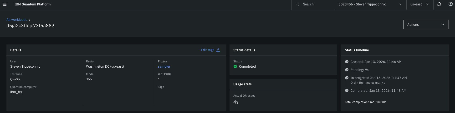
The heatmap above shows the empirical joint distribution over registers a and b. If A and B were independent, the distribution would factor as P(a)P(b) and appear structureless. Instead, probability mass concentrates along a diagonal modular ridge consistent with the interference relation a ≡ k' b (mod 2^n) with k' = 19. Despite heavy noise and near-uniform marginals, localized high-density points align intermittently along this diagonal, forming a delocalized ridge rather than a single contiguous line. This indicates a non-factorizable joint structure in which the signal is encoded geometrically in the correlation pattern, not in either register alone.

The recovered k’ votes histogram above shows the distribution of candidate slopes k′ recovered from joint samples using only invertible values of b. A clear dominant peak appears at k′ = 19, matching the true masked slope used in the circuit, while all other candidates form a lower, noisy background. In the absence of structure, the spectrum would be approximately flat. The presence of a unique global maximum at k′ = 19 indicates that the modular interference relation is globally detectable from joint correlations, even though the true secret k remains hidden by the mask r. Secondary peaks (k′ = 12) reflect finite-shot noise and hardware-induced aliasing.

The Line-Score Spectrum above evaluates every possible slope k′ ∈ ℤ₃₂ by summing the probability mass lying on the corresponding modular line in the joint distribution. In unstructured (independent) data, this profile would be approximately flat. Instead, a pronounced global maximum appears at k′ = 19, indicating a coherent linear interference constraint in the data. There is a prominent secondary peak at k′ = 12, but most candidates are suppressed, reflecting finite-shot noise and hardware-induced broadening rather than independent structure. The result shows that the joint distribution is organized by a global modular relation, not by local coincidences.

The Residual Histogram above collapses the joint distribution along the recovered slope k′. If the slope is correct, residuals concentrate near zero, if incorrect, they spread uniformly. A strong spike at res = 0 and structured side-lobes indicate that the modular relation has been correctly identified. The mutual information MI(A;B) ≈ 0.736 bits quantifies the dependence between registers under the masked-slope encoding. This value confirms the presence of coherent global structure while remaining far below the level required to reconstruct the true secret k without the mask r.

The SVD Spectrum above shows how many independent modes contribute to the joint correlation structure. A rank-1 matrix would indicate a single classical correlation, while a slowly decaying spectrum indicates distributed global structure. Here, the singular values decay smoothly with no sharp cutoff. The first few modes carry significant weight, but many higher modes remain non-negligible. This implies that the interference ridge is not a single classical line, but a superposition of many coherent modes, and that the correlation structure is genuinely high-rank rather than compressible into a low-dimensional classical model.

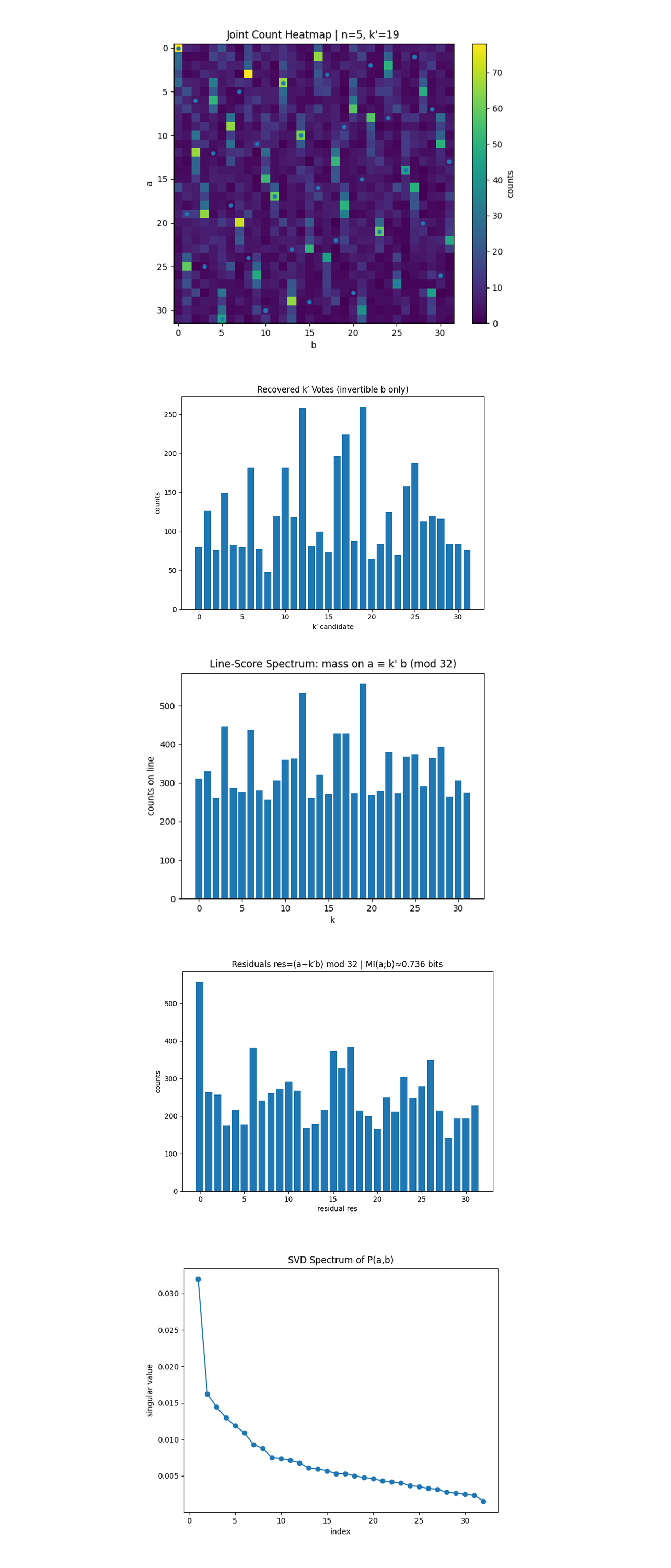
The Cumulative SVD Energy above shows whether the joint distribution P(a,b) is effectively low-rank or high-rank. If the structure were dominated by a single classical constraint, the first one or two singular values would capture most of the energy. Instead, the energy accumulates gradually, with no sharp cutoff, and only approaches saturation after roughly 25 - 30 modes. This indicates that the correlation structure is genuinely high-dimensional, with the interference ridge distributed across many coherent components rather than concentrated in a single dominant mode. The joint distribution is therefore not well-approximated by a rank-1/low-rank factorization (not reducible to P(A)P(B) plus a single dominant mode).

The 2D FFT heatmap above shows the magnitude of the two-dimensional Fourier transform of P(a,b), moving from configuration space to frequency space. A straight modular ridge a ≡ k′ b (mod 32) corresponds to a localized peak at a conjugate frequency pair (ω_a,ω_b). In unstructured or purely noisy data, spectral energy would be broadly distributed. Instead, the spectrum exhibits an isolated Fourier spike, indicating a coherent linear phase structure rather than diffuse statistical noise. This shows that the modular interference relation survives as a well-defined Fourier mode, and that the signal is encoded spectrally in phase coherence, not merely in amplitude bias.

The Per-b Conditional Entropy H(A ∣ B = b) above shows how uncertain A remains when a specific value of B = b is known. In the absence of correlation, the entropy would be flat at log_2 32 = 5 bits, while strong local structure would produce sharp reductions for certain b. Instead, the entropy remains high and nearly uniform, around 4 - 4.5 bits for all b, indicating that no individual column reveals significant information about A. This confirms that the correlation structure is not localized in any single conditional distribution but only emerges globally when many b values are combined.

The Per-b Information Gain above shows the per-column information gain, quantified as the KL divergence D_KL(P(A∣b) ∥ P(A)), measuring how much conditioning on a given b shifts the distribution of A relative to its marginal. The information gain is moderate and broadly distributed across all b, with prominent local peaks (notably at b = 7 and b = 19) but no extreme outliers. This indicates that while some columns carry slightly stronger bias, the correlation signal is not concentrated in a small subset of values. The joint structure therefore cannot be recovered from any single conditional distribution and only emerges from the global geometry of P(a,b).

The Top-120 Joint Outcomes plot above shows the highest-weight joint outcomes (a,b), with the modular ridge a ≡ k' b (mod 32) overlaid. Rather than collapsing onto a single sharp line, the dominant points cluster around the correct diagonal while remaining spatially diffuse. This indicates that the joint distribution organizes geometrically along the true slope, but with phase smearing and noise spreading the support across nearby values. An alternative candidate slope (k′ = 12) partially overlaps the structure but does not dominate, consistent with finite-shot noise and hardware-induced mixing.

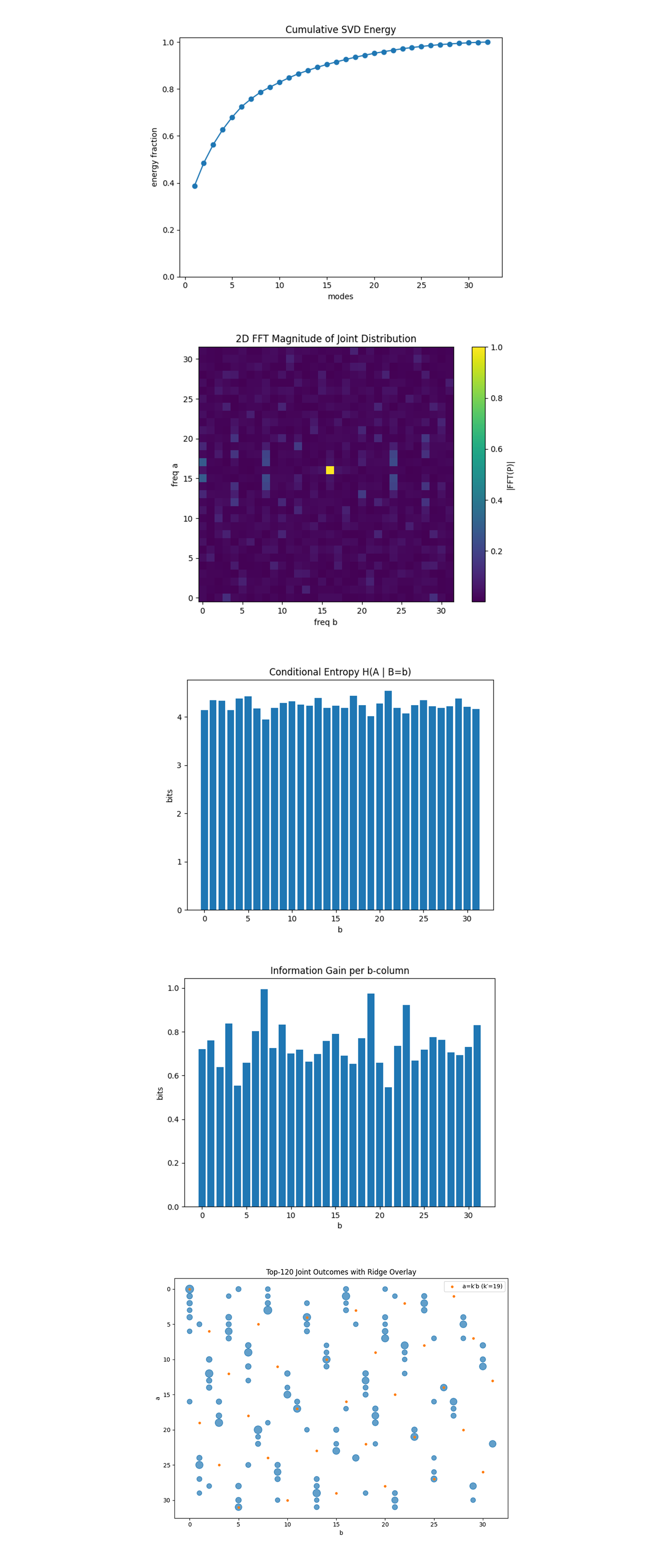
Significance Test of Run Data
Peak line-mass at k'=19: real=557.0 | null mean=268.1 std=64.2 | z=4.50 | p≈0.0033
MI(A;B): real=0.7363 bits | indep-null mean=0.0868 std=0.0039 | z=164.58 | p≈0.0033

The line-score spectrum above provides a direct geometric diagnostic for modular structure by measuring how much probability mass lies on each candidate relation a ≡ k′ b (mod 32). In the real hardware data, a unique global maximum appears at k′ = 19, accumulating significantly more mass than expected under independence. A permutation null test yields a null mean of 268.1±64.2, while the real peak reaches 557 counts, corresponding to a z-score of 4.50 and p ≈ 0.0033. In contrast, both null controls behave as expected, the column-shuffled distribution destroys slope alignment and produces a noisy, structureless spectrum, while the product baseline P(A)P(B) yields an essentially flat profile centered near the uniform expectation. This confirms that the observed ridge is not an artifact of marginal biases or uneven sampling, but a statistically significant global modular alignment present only in the real joint distribution.

The 2D FFT of real joint distribution above shows the magnitude of the two-dimensional Fourier transform of the real joint distribution P(a,b) after removing the DC component. The spectrum exhibits localized off-axis peaks rather than diffuse spectral energy, indicating coherent frequency components associated with a linear coupling between a and b. Such localized spectral features are the Fourier-space signature of a modular ridge in configuration space and demonstrate that the correlation structure persists as a phase-coherent interference pattern rather than a purely statistical amplitude bias.

The 2D FFT after shuffling above columns shows the Fourier magnitude after shuffling columns of the joint distribution, which preserves the marginals P(A) and P(B) but destroys any global slope alignment. In frequency space, the off-axis spectral features associated with the modular ridge disappear, leaving primarily axis-aligned structure. The dominant horizontal band reflects the preserved marginal P(A) and corresponds to separable, one-dimensional statistics rather than nonlocal coupling. The absence of diagonal or slope-dependent spectral peaks confirms that the modular interference geometry has been eliminated by the shuffle.

The product baseline above provides a reference for complete independence. Its Fourier spectrum exhibits only the trivial cross pattern expected from separable marginals, a vertical line from P(B), a horizontal line from P(A), and no off-axis structure. The stark contrast with the real data demonstrates that the spectral features observed there cannot be factorized into independent contributions from A and B, reinforcing the conclusion that the ciphertext is encoded in non-separable joint geometry.

The mutual information between A and B in the real data above is measured to be 0.736 bits, far exceeding the independence-resampling null constructed from the empirical marginals P(A) and P(B), which is tightly clustered around 0.087 bits. This separation is not a finite-shot artifact, the observed value lies many null standard deviations above the baseline, indicating strong non-independent structure in the joint distribution. At the same time, the mutual information remains well below its maximum possible value, quantifying controlled leakage, the joint distribution contains recoverable global structure without directly revealing the masked secret.

The complementary permutation test above focuses specifically on the ridge by examining the probability mass concentrated on each candidate modular line under column shuffling. The resulting null distribution is centered at approximately 268 counts with substantial spread, whereas the real data produces a pronounced peak of 557 counts at k′ = 19. This peak lies approximately 4.5 null standard deviations above the shuffle-null mean. Under a permutation test with 300 random shuffles, the observed line-mass at k′ = 19 exceeds all values observed in the null ensemble, yielding a Monte Carlo p-value of p ≤ 1/(300+1) ≈ 0.0033, the minimum resolvable value under this test.

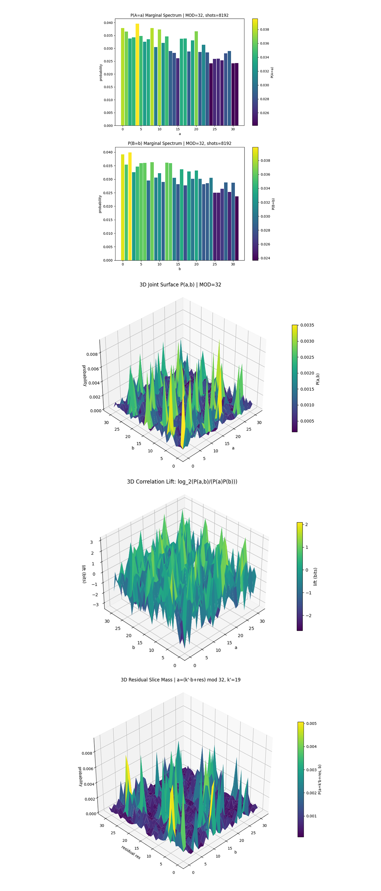
The marginal distribution P(A = a) above is close to uniform, with only mild fluctuations around the expected flat value 1/32. There is no visible structure or periodicity that would hint at k′. An observer with access only to register A sees a statistically generic distribution, indicating that no meaningful information about the masked key is locally encoded in P(A). A slight global slope is visible, with lower values of a occurring more often, consistent with hardware readout bias and amplitude damping favoring low-energy computational states rather than with any structure related to k′. The residual variations are consistent with finite-shot noise and hardware imperfections rather than with an encoded signal.

The marginal distribution P(B = b) above is likewise close to uniform, with only mild fluctuations around the expected flat value 1/32. These variations are unstructured and show no linear or modular pattern that could reveal k′. Importantly, even though b is the register that multiplies k′ inside the arithmetic layer, this dependence is completely washed out at the marginal level. A similar global downward slope appears across b, attributable to systematic hardware bias toward low-Hamming-weight states and not to any modular or key-dependent encoding. Knowing b alone provides no leverage, reinforcing the nonlocal nature of the encoding and preventing either register from acting as a leakage channel.

The 3D joint surface P(a,b) above shows that, unlike the marginals, the joint distribution is highly structured, with sharp localized peaks and ridge-like features that do not factor into P(A)P(B). Probability mass is coherently concentrated along specific joint configurations, even though neither axis alone carries that structure. This directly demonstrates the core phenomenon that the ciphertext is encoded in a joint interference geometry rather than in a classical correlation stored in a single register. The circuit imposes a global constraint that is only visible in the full (a,b) space.

The 3D Correlation Lift above highlights where joint outcomes occur more frequently (positive lift) or less frequently (negative lift) than predicted under independence. The alternating peaks and valleys indicate structured, phase-coherent correlations rather than simple clustering or marginal bias. This shows explicitly that the signal is not merely uneven probability mass, but information gain that exists only at the joint level. In information-theoretic terms, the ciphertext is encoded in the nonzero correlation lift across the (a,b) space.

The 3D residual slice mass above shows the geometry of the interference ridge by projecting the joint distribution onto candidate linear relations of the form a ≡ k′ b + r (mod 32). For the true slope k′ = 19, probability mass concentrates along a coherent ridge across residual offsets res, indicating a global modular structure rather than a localized coincidence. The ridge persists across residual values, demonstrating that the correlation is delocalized and not tied to any single offset or basis. This shows that k′ is recoverable only by reconstructing the full joint geometry and performing coherent post-processing on the joint distribution.

Conclusion

In the end, This experiment implements a toy-scale interference-based encryption scheme on real IBM quantum hardware. A masked secret scalar k is encoded into a joint quantum state over registers a and b using a group-phase construction over ℤ₃₂, without ever being stored in any single register. Instead, the ciphertext appears only as a global modular interference relation a ≡ k′ b (mod 32), recoverable exclusively from joint measurement statistics. Across 8192 shots, the experiment produces a stable interference ridge in the 32 x 32 outcome space, while all marginals remain statistically close to uniform. A battery of geometric, spectral, and information-theoretic diagnostics confirms that the signal exists as a delocalized, phase-coherent joint structure rather than a classical correlation or marginal artifact. Recovering k′ requires reconstructing the full joint geometry, after which unmasking yields the true secret k. These results demonstrate that even at small scale, quantum interference can encode information in a form that is globally accessible yet locally hidden, suggesting a principled route toward nonlocal cryptographic primitives based on joint structure rather than local observables. All code, circuits, visualizations, and raw backend results are available at https://github.com/SteveTipp/Qwork.github.io or via the project website www.qubits.work.

Code:


# Main circuit
# Imports
import os, json, logging, math
from datetime import datetime
from collections import Counter
import pandas as pd
from qiskit import QuantumCircuit, transpile
from qiskit_ibm_runtime import QiskitRuntimeService, SamplerV2 as Sampler

# Logging
logging.basicConfig(level=logging.INFO, format="%(asctime)s | %(levelname)s | %(message)s")
log = logging.getLogger(__name__)

# IBMQ
TOKEN = "YOUR_IBMQ_API_KEY"
INSTANCE = "YOUR_IBMQ_CRN"
BACKEND_NAME = "ibm_fez"
CAL_CSV = "MOST_RECENT_ibm_fez_calibrations.csv"
SHOTS = 8192

# Parameters (toy nonlocal ridge encryption. Ciphertext slope k' = k + r mod 2^n)
N_BITS = 5
N_MOD = 1 << N_BITS
K_SECRET = 13
R_MASK = 6
K_PRIME = (K_SECRET + R_MASK) % N_MOD

if K_PRIME % 2 == 0:
    raise ValueError("K_PRIME must be odd (invertible mod 2^n). Pick different K_SECRET/R_MASK.")

log.info(f"n={N_BITS} | k={K_SECRET} | r={R_MASK} | k'={K_PRIME}")

# QFT/iQFT (little-endian qubit order. Qubits[0] = LSB)
def qft(qc: QuantumCircuit, qubits: list[int]) -> None:
    n = len(qubits)
    for j in range(n):
        qc.h(qubits[j])
        for k in range(j + 1, n):
            angle = math.pi / (1 << (k - j))
            qc.cp(angle, qubits[k], qubits[j])
    for i in range(n // 2):
        qc.swap(qubits[i], qubits[n - 1 - i])

def iqft(qc: QuantumCircuit, qubits: list[int]) -> None:
    n = len(qubits)
    for i in range(n // 2):
        qc.swap(qubits[i], qubits[n - 1 - i])
    for j in reversed(range(n)):
        for k in reversed(range(j + 1, n)):
            angle = -math.pi / (1 << (k - j))
            qc.cp(angle, qubits[k], qubits[j])
        qc.h(qubits[j])

# Constant multiply a = (k * b) mod 2^n using QFT adder (b in computational basis, a in Fourier basis)
def const_mul_mod_2n(qc: QuantumCircuit, a: list[int], b: list[int], k: int) -> None:
    n = len(a)
    qft(qc, a)
    for bj in range(n):
        c = (k << bj) % (1 << n)
        if c == 0:
            continue
        for ak in range(n):
            angle = (2.0 * math.pi * c) / (1 << (ak + 1))
            qc.cp(angle, b[bj], a[ak])
    iqft(qc, a)

# Circuit (ciphertext lives in joint (a,b) correlation: a = k' * b mod 2^n)
a = list(range(N_BITS))
b = list(range(N_BITS, 2 * N_BITS))
qc = QuantumCircuit(2 * N_BITS, 2 * N_BITS)

qc.h(b)
const_mul_mod_2n(qc, a, b, K_PRIME)
qc.measure(range(2 * N_BITS), range(2 * N_BITS))

# Calibration based qubit pick 
def best_qubits(csv_path: str, n: int) -> list[int]:
    df = pd.read_csv(csv_path)
    df.columns = df.columns.str.strip()
    winners = (
        df.sort_values(["√x (sx) error", "T1 (us)", "T2 (us)"],
                       ascending=[True, False, False])
        ["Qubit"].head(n).tolist()
    )
    log.info("Best physical qubits: %s", winners)
    return winners

PHYSICAL = best_qubits(CAL_CSV, 2 * N_BITS)

# IBM Runtime  
service = QiskitRuntimeService(channel="ibm_cloud", token=TOKEN, instance=INSTANCE)
backend = service.backend(BACKEND_NAME)
log.info("Backend → %s", backend.name)

trans = transpile(qc,
                  backend=backend,
                  initial_layout=PHYSICAL,
                  optimization_level=3)
log.info("Circuit depth %d, gate counts %s", trans.depth(), trans.count_ops())

# SamplerV2
sampler = Sampler(mode=backend)
job = sampler.run([trans], shots=SHOTS)
result = job.result()

# Classical post processing (recover k' from joint stats and unblind k with r)
creg_name = trans.cregs[0].name
counts_raw = result[0].data.__getattribute__(creg_name).get_counts()

def _split_ab(bs: str, nbits: int) -> tuple[int, int]:
    s = bs.replace(" ", "")[::-1]
    aval = int(s[0:nbits][::-1], 2)
    bval = int(s[nbits:2*nbits][::-1], 2)
    return aval, bval

def invert_mod_2n_odd(x: int, nbits: int) -> int:
    if x % 2 == 0:
        raise ValueError("No inverse for even numbers mod 2^n.")
    mod = 1 << nbits
    inv = 1
    for _ in range(nbits):
        inv = (inv * (2 - x * inv)) % mod
    return inv

A = Counter()
B = Counter()
votes = Counter()

for bs, cts in counts_raw.items():
    aval, bval = _split_ab(bs, N_BITS)
    A[aval] += cts
    B[bval] += cts
    if bval % 2 == 1:
        invb = invert_mod_2n_odd(bval, N_BITS)
        votes[(aval * invb) % N_MOD] += cts

k_prime_hat = votes.most_common(1)[0][0] if votes else None
k_secret_hat = (k_prime_hat - R_MASK) % N_MOD if k_prime_hat is not None else None

log.info("Marginals | A_unique=%d B_unique=%d (expect near %d)", len(A), len(B), N_MOD)
log.info("Recovered k' (attacker sees) = %s (true %d)", str(k_prime_hat), K_PRIME)
log.info("Unblinded k (needs r)        = %s (true %d)", str(k_secret_hat), K_SECRET)

# Save JSON
out = {
    "experiment": "Nonlocal_Ridge_Encryption_n5",
    "backend": backend.name,
    "physical_qubits": PHYSICAL,
    "shots": SHOTS,
    "calibration_csv": CAL_CSV,
    "n_bits": N_BITS,
    "modulus": N_MOD,
    "k_secret": K_SECRET,
    "r_mask": R_MASK,
    "k_prime_cipher": K_PRIME,
    "k_prime_hat": k_prime_hat,
    "k_secret_hat": k_secret_hat,
    "marginals": {"A_counts": dict(A), "B_counts": dict(B)},
    "k_prime_votes_top10": votes.most_common(10),
    "counts": counts_raw
}

JSON_PATH = "FILE_PATH_TO_SAVE_BACKEND_RESULT_JSON.json"
with open(JSON_PATH, "w") as fp:
    json.dump(out, fp, indent=4)
log.info("Results saved → %s", JSON_PATH)

# End

# Code for all visuals from experiment JSON
# Imports
import json
from collections import Counter
from math import gcd, log2
import numpy as np
import matplotlib.pyplot as plt
from mpl_toolkits.mplot3d import Axes3D  

# Load Run data
FILE_PATH = "FILE_PATH_TO_IMPORT_BACKEND_RESULT_JSON.json"

with open(FILE_PATH, "r") as f:
    data = json.load(f)

counts_raw = data["counts"]
N = int(data["n_bits"])          
MOD = int(data["modulus"])       
shots = int(data["shots"])

# Handle naming differences safely
k_prime = int(data.get("k_prime_hat", data.get("k_prime_cipher")))

# Parse bitstrings -> (a, b)
def parse_ab(bitstring: str):
    s = bitstring.replace(" ", "")[::-1]
    a = int(s[0:N][::-1], 2)
    b = int(s[N:2 * N][::-1], 2)
    return a, b

# Build counters and joint count matrix
joint = Counter()
A = Counter()
B = Counter()
total = 0

for bitstring, c in counts_raw.items():
    a, b = parse_ab(bitstring)
    joint[(a, b)] += c
    A[a] += c
    B[b] += c
    total += c

assert total == shots

C = np.zeros((MOD, MOD), dtype=np.int64)
for (a, b), c in joint.items():
    C[a, b] = c

P = C / max(total, 1)   
pA = P.sum(axis=1)      
pB = P.sum(axis=0)      

bb = np.arange(MOD)
aa = (k_prime * bb) % MOD

# Joint heatmap and ridge overlay
plt.figure()
plt.imshow(C)
plt.title(f"Joint Count Heatmap | n={N}, k'={k_prime}")
plt.xlabel("b")
plt.ylabel("a")
plt.colorbar(label="counts")

plt.scatter(bb, aa, s=18)
plt.show()

# k' vote histogram from invertible b
votes = Counter()
invertible_mass = 0

for (a, b), c in joint.items():
    if gcd(b, MOD) == 1:
        inv_b = pow(b, -1, MOD)
        k_cand = (a * inv_b) % MOD
        votes[k_cand] += c
        invertible_mass += c

plt.figure()
plt.bar(range(MOD), [votes[k] for k in range(MOD)])
plt.title("Recovered k′ Votes (invertible b only)")
plt.xlabel("k′ candidate")
plt.ylabel("counts")
plt.show()

# Line-score spectrum
line_mass = []
for k in range(MOD):
    m = 0
    for (a, b), c in joint.items():
        if (a - k * b) % MOD == 0:
            m += c
    line_mass.append(m)

plt.figure()
plt.bar(range(MOD), line_mass)
plt.title("Line-Score Spectrum: mass on a ≡ k' b (mod 32)")
plt.xlabel("k")
plt.ylabel("counts on line")
plt.show()

# Residual histogram and mutual information
residual = [0] * MOD
for (a, b), c in joint.items():
    r = (a - k_prime * b) % MOD
    residual[r] += c

mi = 0.0
for (a, b), c in joint.items():
    p_ab = c / total
    mi += p_ab * log2(p_ab / ((A[a] / total) * (B[b] / total)))

plt.figure()
plt.bar(range(MOD), residual)
plt.title(f"Residuals res=(a−k′b) mod 32 | MI(a;b)≈{mi:.3f} bits")
plt.xlabel("residual res")
plt.ylabel("counts")
plt.show()

# SVD spectrum
U, S, Vt = np.linalg.svd(P, full_matrices=False)
energy = (S**2) / np.sum(S**2)
cum_energy = np.cumsum(energy)

plt.figure()
plt.plot(np.arange(1, len(S) + 1), S, marker="o")
plt.title("SVD Spectrum of P(a,b)")
plt.xlabel("index")
plt.ylabel("singular value")
plt.show()

plt.figure()
plt.plot(np.arange(1, len(S) + 1), cum_energy, marker="o")
plt.title("Cumulative SVD Energy")
plt.xlabel("modes")
plt.ylabel("energy fraction")
plt.ylim(0, 1.02)
plt.show()

# 2D FFT magnitude
F = np.fft.fftshift(np.fft.fft2(P))
plt.figure()
plt.imshow(np.abs(F), origin="lower")
plt.colorbar(label="|FFT(P)|")
plt.title("2D FFT Magnitude of Joint Distribution")
plt.xlabel("freq b")
plt.ylabel("freq a")
plt.show()

# Conditional entropy H(A|b)
eps = 1e-15
H_A_given_b = np.zeros(MOD)

for b in range(MOD):
    if pB[b] > 0:
        col = P[:, b] / pB[b]
        H_A_given_b[b] = -np.sum(col * np.log2(np.maximum(col, eps)))

plt.figure()
plt.bar(range(MOD), H_A_given_b)
plt.title("Conditional Entropy H(A | B=b)")
plt.xlabel("b")
plt.ylabel("bits")
plt.show()

# KL divergence D(P(A|b) || P(A))
KL_col = np.zeros(MOD)
for b in range(MOD):
    if pB[b] > 0:
        pA_given_b = P[:, b] / pB[b]
        KL_col[b] = np.sum(
            pA_given_b * np.log2(np.maximum(pA_given_b / np.maximum(pA, eps), eps))
        )

plt.figure()
plt.bar(range(MOD), KL_col)
plt.title("Information Gain per b-column")
plt.xlabel("b")
plt.ylabel("bits")
plt.show()

# Top-mass constellation and ridge overlays
flat = [(C[a, b], a, b) for a in range(MOD) for b in range(MOD) if C[a, b] > 0]
flat.sort(reverse=True)

TOPN = min(120, len(flat))
top = flat[:TOPN]

sizes = 20 + 180 * (np.array([x[0] for x in top]) / top[0][0])**0.8
a_top = [x[1] for x in top]
b_top = [x[2] for x in top]

plt.figure()
plt.scatter(b_top, a_top, s=sizes, alpha=0.7)
plt.scatter(bb, aa, s=12, label=f"a=k′b (k′={k_prime})")
plt.gca().invert_yaxis()
plt.title(f"Top-{TOPN} Joint Outcomes with Ridge Overlay")
plt.xlabel("b")
plt.ylabel("a")
plt.legend()
plt.show()

# Controls and Significance
def mutual_information_from_C(Cmat: np.ndarray) -> float:
    """MI(A;B) in bits from count matrix C[a,b]."""
    total_local = int(np.sum(Cmat))
    if total_local <= 0:
        return 0.0

    Pm = Cmat / total_local
    pA_ = Pm.sum(axis=1, keepdims=True)
    pB_ = Pm.sum(axis=0, keepdims=True)

    eps_ = 1e-15
    denom = np.maximum(pA_ * pB_, eps_)
    ratio = Pm / denom

    mask = Pm > 0
    return float(np.sum(Pm[mask] * np.log2(np.maximum(ratio[mask], eps_))))

def line_mass_spectrum_from_C(Cmat: np.ndarray, mod: int) -> np.ndarray:
    """For each slope k, mass on line a ≡ k b (mod mod)."""
    out = np.zeros(mod, dtype=np.int64)
    for k in range(mod):
        m = 0
        for b in range(mod):
            a = (k * b) % mod
            m += int(Cmat[a, b])
        out[k] = m
    return out

def shuffle_columns(Cmat: np.ndarray, rng: np.random.Generator) -> np.ndarray:
    """Shuffle columns of C (permute b labels). Preserves row/col sums exactly."""
    perm = rng.permutation(Cmat.shape[1])
    return Cmat[:, perm]

def safe_hist(ax, x: np.ndarray, bins: int = 30):
    """
    Histogram that won't crash if x has (near) zero range.
    Falls back to a single bin/bar if needed.
    """
    x = np.asarray(x, dtype=float)
    xmin, xmax = float(np.min(x)), float(np.max(x))
    if np.isclose(xmin, xmax):
        ax.bar([xmin], [len(x)], width=0.0001 if xmin != 0 else 0.0001)
        ax.set_xlim(xmin - 0.001, xmax + 0.001)
        return

    rng = xmax - xmin
    if rng < 1e-6:
        bins = 5

    ax.hist(x, bins=bins)

# Product baseline P(A)P(B) turned into a counts-like matrix
C_prod = np.outer(pA, pB) * total  # expected counts under independence
C_prod = np.rint(C_prod).astype(np.int64)

# Ridge alignment control
rng = np.random.default_rng(7)
C_shuf_example = shuffle_columns(C, rng)

# Line-score comparison real vs shuffled vs product
line_real = line_mass_spectrum_from_C(C, MOD)
line_shuf = line_mass_spectrum_from_C(C_shuf_example, MOD)
line_prod = line_mass_spectrum_from_C(C_prod, MOD)

plt.figure()
plt.plot(range(MOD), line_real, marker="o", label="real")
plt.plot(range(MOD), line_shuf, marker="o", label="shuffled columns (alignment null)")
plt.plot(range(MOD), line_prod, marker="o", label="P(A)P(B) baseline")
plt.title("Line-Score Comparison (real vs null controls)")
plt.xlabel("k")
plt.ylabel("counts on a ≡ k' b (mod 32)")
plt.legend()
plt.show()

def fft_mag(Pmat: np.ndarray) -> np.ndarray:
    Fm = np.fft.fftshift(np.fft.fft2(Pmat))
    return np.abs(Fm)

P_real = C / max(total, 1)
P_shuf = C_shuf_example / max(total, 1)
P_prod = C_prod / max(total, 1)

F_real = fft_mag(P_real)
F_shuf = fft_mag(P_shuf)
F_prod = fft_mag(P_prod)

# Remove DC for visualization
center = MOD // 2
F_real_vis = F_real.copy()
F_real_vis[center, center] = 0
F_shuf_vis = F_shuf.copy()
F_shuf_vis[center, center] = 0
F_prod_vis = F_prod.copy()
F_prod_vis[center, center] = 0

plt.figure()
plt.imshow(F_real_vis, origin="lower")
plt.colorbar(label="|FFT| (DC removed)")
plt.title("FFT Magnitude | real P(a,b)")
plt.xlabel("freq b")
plt.ylabel("freq a")
plt.show()

plt.figure()
plt.imshow(F_shuf_vis, origin="lower")
plt.colorbar(label="|FFT| (DC removed)")
plt.title("FFT Magnitude | shuffled-column null")
plt.xlabel("freq b")
plt.ylabel("freq a")
plt.show()

plt.figure()
plt.imshow(F_prod_vis, origin="lower")
plt.colorbar(label="|FFT| (DC removed)")
plt.title("FFT Magnitude | P(A)P(B) baseline")
plt.xlabel("freq b")
plt.ylabel("freq a")
plt.show()

# Significance tests
NUM_PERM = 300
k0 = int(k_prime) % MOD
peak_real = float(line_real[k0])
mi_real = mutual_information_from_C(C)

# Ridge-line null via column shuffles
peak_null = np.zeros(NUM_PERM, dtype=float)
rng = np.random.default_rng(123)
for i in range(NUM_PERM):
    C_sh = shuffle_columns(C, rng)
    line_sh = line_mass_spectrum_from_C(C_sh, MOD)
    peak_null[i] = float(line_sh[k0])

# MI null via independent resampling from marginals
mi_null = np.zeros(NUM_PERM, dtype=float)

pA_norm = pA / max(np.sum(pA), 1e-15)
pB_norm = pB / max(np.sum(pB), 1e-15)

rng_mi = np.random.default_rng(999)
for i in range(NUM_PERM):
    a_samp = rng_mi.choice(MOD, size=total, p=pA_norm)
    b_samp = rng_mi.choice(MOD, size=total, p=pB_norm)

    C_ind = np.zeros((MOD, MOD), dtype=np.int64)
    np.add.at(C_ind, (a_samp, b_samp), 1)

    mi_null[i] = mutual_information_from_C(C_ind)

# p-values 
p_peak = (np.sum(peak_null >= peak_real) + 1) / (NUM_PERM + 1)
p_mi = (np.sum(mi_null >= mi_real) + 1) / (NUM_PERM + 1)

# z-scores
pk_mu, pk_sig = float(np.mean(peak_null)), float(np.std(peak_null) + 1e-12)
mi_mu, mi_sig = float(np.mean(mi_null)), float(np.std(mi_null) + 1e-12)
z_peak = (peak_real - pk_mu) / pk_sig
z_mi = (mi_real - mi_mu) / mi_sig

print("\nSignificance Tests")
print(
    f"Peak line-mass at k'={k0}: real={peak_real:.1f} | null mean={pk_mu:.1f} std={pk_sig:.1f} "
    f"| z={z_peak:.2f} | p≈{p_peak:.4f}"
)
print(
    f"MI(A;B): real={mi_real:.4f} bits | indep-null mean={mi_mu:.4f} std={mi_sig:.4f} "
    f"| z={z_mi:.2f} | p≈{p_mi:.4f}"
)

# Visualize null distributions
fig, ax = plt.subplots()
safe_hist(ax, mi_null, bins=30)
ax.axvline(mi_real, linestyle="--", linewidth=2, label="real MI")
ax.set_title("MI Null (independence resampling from P(A)P(B))")
ax.set_xlabel("MI (bits)")
ax.set_ylabel("count")
ax.legend()
plt.show()

fig, ax = plt.subplots()
safe_hist(ax, peak_null, bins=30)
ax.axvline(peak_real, linestyle="--", linewidth=2, label=f"real peak at k'={k0}")
ax.set_title("Peak Line-Mass Null (column-shuffle alignment test)")
ax.set_xlabel("counts on ridge line")
ax.set_ylabel("count")
ax.legend()
plt.show()

# Bar-spectrum of P(A=a)
cmap = plt.cm.viridis
x_a = np.arange(MOD)
norm_a = plt.Normalize(vmin=np.min(pA), vmax=np.max(pA))
colors_a = cmap(norm_a(pA))

fig, ax = plt.subplots()
ax.bar(x_a, pA, color=colors_a, width=0.9)

sm_a = plt.cm.ScalarMappable(cmap=cmap, norm=norm_a)
sm_a.set_array([])
fig.colorbar(sm_a, ax=ax, label="P(A=a)")

ax.set_title(f"P(A=a) Marginal Spectrum | MOD={MOD}, shots={shots}")
ax.set_xlabel("a")
ax.set_ylabel("probability")
plt.tight_layout()
plt.show()

# Bar-spectrum of P(B=b)
x_b = np.arange(MOD)
norm_b = plt.Normalize(vmin=np.min(pB), vmax=np.max(pB))
colors_b = cmap(norm_b(pB))

fig, ax = plt.subplots()
ax.bar(x_b, pB, color=colors_b, width=0.9)

sm_b = plt.cm.ScalarMappable(cmap=cmap, norm=norm_b)
sm_b.set_array([])
fig.colorbar(sm_b, ax=ax, label="P(B=b)")

ax.set_title(f"P(B=b) Marginal Spectrum | MOD={MOD}, shots={shots}")
ax.set_xlabel("b")
ax.set_ylabel("probability")
plt.tight_layout()
plt.show()

# Shared mesh for 3D surfaces
Agrid, Bgrid = np.meshgrid(np.arange(MOD), np.arange(MOD), indexing="ij")

# 3D surface of the joint distribution P(a,b) 
fig = plt.figure()
ax = fig.add_subplot(111, projection="3d")
surf = ax.plot_surface(
    Agrid, Bgrid, P,
    rstride=1, cstride=1,
    linewidth=0, antialiased=True,
    cmap="viridis",
)
fig.colorbar(surf, ax=ax, shrink=0.6, pad=0.08, label="P(a,b)")
ax.set_title(f"3D Joint Surface P(a,b) | MOD={MOD}")
ax.set_xlabel("a")
ax.set_ylabel("b")
ax.set_zlabel("probability")
ax.view_init(elev=35, azim=-135)
plt.tight_layout()
plt.show()

# 3D surface of correlation lift
eps = 1e-15
pA_mat = pA[:, None]
pB_mat = pB[None, :]
indep = np.clip(pA_mat * pB_mat, eps, None)
ratio = np.clip(P / indep, eps, None)
lift = np.log2(ratio)

# Mask places where P is zero to avoid huge negative floors
lift_masked = np.where(P > 0, lift, np.nan)

fig = plt.figure()
ax = fig.add_subplot(111, projection="3d")
surf = ax.plot_surface(
    Agrid, Bgrid, lift_masked,
    rstride=1, cstride=1,
    linewidth=0, antialiased=True,
    cmap="viridis",
)
fig.colorbar(surf, ax=ax, shrink=0.6, pad=0.08, label="lift (bits)")
ax.set_title("3D Correlation Lift: log_2(P(a,b)/(P(a)P(b)))")
ax.set_xlabel("a")
ax.set_ylabel("b")
ax.set_zlabel("lift (bits)")
ax.view_init(elev=35, azim=-135)
plt.tight_layout()
plt.show()

# 3D residual-conditioned ridge mass
R = np.zeros((MOD, MOD), dtype=np.float64)  # rows=b, cols=r
for b in range(MOD):
    for r in range(MOD):
        a = (k_prime * b + r) % MOD
        R[b, r] = P[a, b]

BB, RR = np.meshgrid(np.arange(MOD), np.arange(MOD), indexing="ij")  # B x R
fig = plt.figure()
ax = fig.add_subplot(111, projection="3d")
surf = ax.plot_surface(
    BB, RR, R,
    rstride=1, cstride=1,
    linewidth=0, antialiased=True,
    cmap="viridis",
)
fig.colorbar(surf, ax=ax, shrink=0.6, pad=0.08, label="P(a=k'b+res, b)")
ax.set_title(f"3D Residual Slice Mass | a=(k'·b+res) mod {MOD}, k'={k_prime}")
ax.set_xlabel("b")
ax.set_ylabel("residual res")
ax.set_zlabel("probability")
ax.view_init(elev=35, azim=-135)
plt.tight_layout()
plt.show()

# End

// Code for Three.js render of backend data
// Config
const HALF_BITS  = 5;                 // 5 per axis
const TOTAL_BITS = 2 * HALF_BITS;     // 10
const GRID       = 1 << HALF_BITS;    // 32
const MOD        = GRID;              // 32

// Nonlocal Ridge Encryption params 
const K_PRIME  = 19;                  // cipher slope (attacker sees) k'
const R_MASK   = 6;                   // one-time mask r
const K_SECRET = ((K_PRIME - R_MASK) % MOD + MOD) % MOD; // 13

// Load JSON
async function loadQuantumData() {
  const res  = await fetch('Nonlocal_Ridge_Encryption_n5_0.json'); 
  const data = await res.json();
  return data.counts; // bitstring -> count
}

// Three.js setup
const scene    = new THREE.Scene();
const camera   = new THREE.PerspectiveCamera(75, window.innerWidth / window.innerHeight, 0.1, 1000);
const renderer = new THREE.WebGLRenderer({ antialias: true });
renderer.setSize(window.innerWidth, window.innerHeight);
document.body.appendChild(renderer.domElement);

// Controls and lighting
const controls = new THREE.OrbitControls(camera, renderer.domElement);
const light = new THREE.DirectionalLight(0xffffff, 1);
light.position.set(10, 10, 10);
scene.add(light);

// Camera
camera.position.set(0, 30, 60);
camera.lookAt(0, 0, 0);

// Globals
let mesh;
let dots = [];
let time = 0;

// Helpers
const padN = (s, n) => s.padStart(n, '0').slice(-n);
const rev  = s => s.split('').reverse().join(''); // mirror Python's bs[::-1]
const mod  = (x, m) => ((x % m) + m) % m;

// Parse into classical (a,b) matching Python bit ordering
function parseEntries(counts) {
  const entries = [];
  for (const [bit, cRaw] of Object.entries(counts)) {
    const b10 = padN(String(bit).replace(/\s+/g, ""), TOTAL_BITS);
    const left  = b10.slice(0, HALF_BITS);    // raw left 5
    const right = b10.slice(HALF_BITS);       // raw right 5

    // Python mapping: a = int(right[::-1],2), b = int(left[::-1],2)
    const a = parseInt(rev(right), 2);
    const b = parseInt(rev(left),  2);

    entries.push({ bit, a, b, count: Number(cRaw) });
  }
  return entries;
}

// Build matrix as heat[a][b] (rows=a, cols=b) 
function buildHeat(entries) {
  const heat = Array.from({ length: GRID }, () => Array(GRID).fill(0));
  let maxCount = 0;
  for (const e of entries) {
    heat[e.a][e.b] = e.count;
    if (e.count > maxCount) maxCount = e.count;
  }
  return { heat, maxCount };
}

// Build surface and dots 
function createWaveSurface(heat, maxCount) {
  const WIDTH    = GRID * 2;
  const SEGMENTS = WIDTH;
  const STEP     = WIDTH / (GRID - 1);

  const geometry = new THREE.PlaneGeometry(WIDTH, WIDTH, SEGMENTS, SEGMENTS);
  const colors   = [];
  const gridX    = SEGMENTS + 1;
  const gridY    = SEGMENTS + 1;

  for (let y = 0; y < gridY; y++) {
    for (let x = 0; x < gridX; x++) {
      // Map geometry samples -> discrete lattice. x-axis = b (cols), y-axis = a (rows)
      const b = Math.min(GRID - 1, Math.floor(x / (gridX / GRID)));
      const a = Math.min(GRID - 1, Math.floor(y / (gridY / GRID)));

      const c   = heat[a]?.[b] ?? 0;
      const amp = maxCount > 0 ? (c / maxCount) : 0;

      // Ridge: a ≡ k' * b (mod 32) 
      const isRidge = mod(a - (K_PRIME * b), MOD) === 0;

      // Ridge lattice points
      const color = isRidge
        ? new THREE.Color(0x0000ff) // ridge cells (blue)
        : new THREE.Color(0x00ff00); // background (green)

      colors.push(color.r, color.g, color.b);
    }
  }

  geometry.setAttribute('color', new THREE.Float32BufferAttribute(colors, 3));
  const material = new THREE.MeshBasicMaterial({ vertexColors: true, wireframe: true });

  mesh = new THREE.Mesh(geometry, material);
  mesh.rotation.x = -Math.PI / 2;

  // Store for animation
  mesh.userData = { heat, maxCount, GRID, STEP, gridX, gridY };
  scene.add(mesh);

  // Red dots ONLY where count > 0 
  const dotMat = new THREE.MeshBasicMaterial({ color: 0xff0000 });
  for (let a = 0; a < GRID; a++) {
    for (let b = 0; b < GRID; b++) {
      const c = heat[a][b];
      if (!c || c <= 0) continue;

      const amp = maxCount > 0 ? (c / maxCount) : 0;

      const dot = new THREE.Mesh(new THREE.SphereGeometry(0.18, 10, 10), dotMat);
      dot.userData = { a, b, amp };

      // x=b, z=a 
      dot.position.set(
        (b - (GRID - 1) / 2) * STEP,
        amp * 20 + 0.6,
        (a - (GRID - 1) / 2) * STEP
      );

      dots.push(dot);
      scene.add(dot);
    }
  }

  console.log(`Nonlocal Ridge Encryption: k'=${K_PRIME}, r=${R_MASK}, k=${K_SECRET}`);
}

// Animate
function animate() {
  requestAnimationFrame(animate);
  time += 0.2;
  if (!mesh) return;

  const { heat, maxCount, GRID, gridX, gridY } = mesh.userData;
  const pos = mesh.geometry.attributes.position;

  for (let i = 0; i < pos.count; i++) {
    const x = i % gridX;
    const y = Math.floor(i / gridX);

    const b = Math.min(GRID - 1, Math.floor(x / (gridX / GRID)));
    const a = Math.min(GRID - 1, Math.floor(y / (gridY / GRID)));

    const c   = heat[a]?.[b] ?? 0;
    const amp = maxCount > 0 ? (c / maxCount) : 0;

    // Wave motion
    const wave = Math.sin((x + time) * 0.4) * Math.cos((y + time) * 0.4);
    pos.setZ(i, amp * wave * 20);
  }

  // Keep dots floating at their amplitude height 
  dots.forEach(dot => {
    dot.position.y = dot.userData.amp * 20 + 0.6;
  });

  pos.needsUpdate = true;
  controls.update();
  renderer.render(scene, camera);
}

// Main
loadQuantumData().then(counts => {
  const entries = parseEntries(counts);
  const { heat, maxCount } = buildHeat(entries);

  createWaveSurface(heat, maxCount);
  animate();
});

// End